系统地综合使用可视化和数据变形来探索数据。EDA(Exploratory Data Analysis)
EDA的循环步骤:
- 针对数据产生问题(假设);
- 通过数据可视化、变形、建模来回答问题(验证假设);
- 用所获得的知识改善问题或产生新问题;
EDA不是一个严格的标准过程,而是一种思维模式。EDA的目的是对数据的理解。
library(tidyverse)## Warning: 程辑包'tidyverse'是用R版本3.5.1 来建造的## Warning: 程辑包'tidyr'是用R版本3.5.1 来建造的## Warning: 程辑包'readr'是用R版本3.5.1 来建造的## Warning: 程辑包'forcats'是用R版本3.5.1 来建造的library(hexbin)## Warning: 程辑包'hexbin'是用R版本3.5.2 来建造的library(modelr)## Warning: 程辑包'modelr'是用R版本3.5.1 来建造的问题
“There are no routine statistical questions, only questionable statistical routines.”
— Sir David Cox
“Far better an approximate answer to the right question, which is often vague, than an exact answer to the wrong question, which can always be made precise.”
— John Tukey
使用问题来引导对数据的理解。EDA是个需要创造力的过程。通过问题来不断深化对数据的理解,越来越能问出好问题。
有两类经典问题:
- 变量的变化是怎样的?(variation)
- 变量之间的协变化是怎样的?(covariation)
Variation
可视化分布
怎样可视化变量的分布取决于变量是离散的还是连续的。
对于分类变量,通常使用柱状图(bar chart)
ggplot(data = diamonds) +
  geom_bar(mapping = aes(x = cut))
或者直接输出计数
diamonds %>%
  count(cut)
## # A tibble: 5 x 2
## cut n
## <ord> <int>
## 1 Fair 1610
## 2 Good 4906
## 3 Very Good 12082
## 4 Premium 13791
## 5 Ideal 21551table(diamonds$cut)##
## Fair Good Very Good Premium Ideal
## 1610 4906 12082 13791 21551对于连续变量,使用直方图(histogram)
ggplot(data = diamonds) +
  geom_histogram(mapping = aes(x = carat), binwidth = 0.5)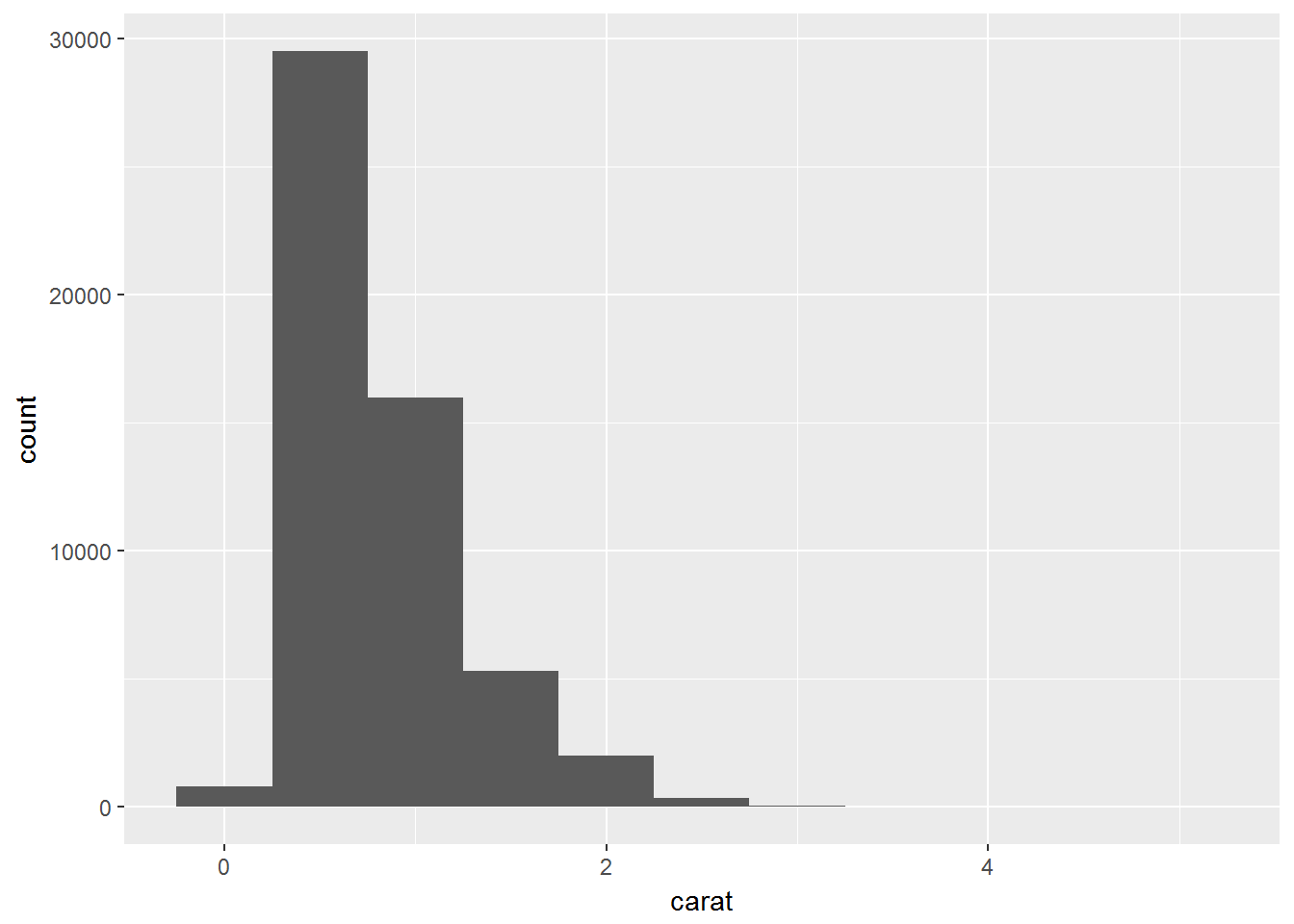
可以手动计算分箱
diamonds %>%
  count(cut_width(carat, 0.5))
## # A tibble: 11 x 2
## `cut_width(carat, 0.5)` n
## <fct> <int>
## 1 [-0.25,0.25] 785
## 2 (0.25,0.75] 29498
## 3 (0.75,1.25] 15977
## 4 (1.25,1.75] 5313
## 5 (1.75,2.25] 2002
## 6 (2.25,2.75] 322
## 7 (2.75,3.25] 32
## 8 (3.25,3.75] 5
## 9 (3.75,4.25] 4
## 10 (4.25,4.75] 1
## 11 (4.75,5.25] 1使用直方图时,应使用多个分箱区间来放大和缩小区间及粒度。
smaller <- diamonds %>%
  filter(carat < 3)

ggplot(data = smaller, mapping = aes(x = carat)) +
  geom_histogram(binwidth = 0.1)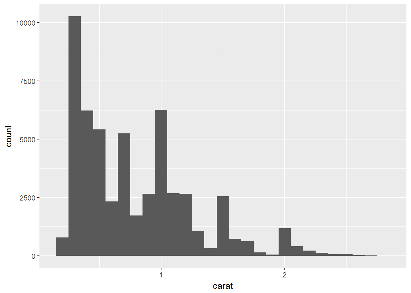
如果想绘制多个直方图(比如一组分类变量下的),则使用geom_freqpoly
ggplot(data = smaller, mapping = aes(x = carat, colour = cut)) +
  geom_freqpoly(binwidth = 0.1)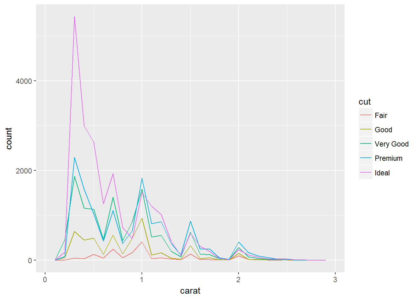
典型值
一些可能的问题:
- Which values are the most common? Why?
- Which values are rare? Why? Does that match your expectations?
- Can you see any unusual patterns? What might explain them?
对于钻石问题来说:
- Why are there more diamonds at whole carats and common fractions of carats?
- Why are there more diamonds slightly to the right of each peak than there are slightly to the left of each peak?
- Why are there no diamonds bigger than 3 carats?
ggplot(data = smaller, mapping = aes(x = carat)) +
  geom_histogram(binwidth = 0.01)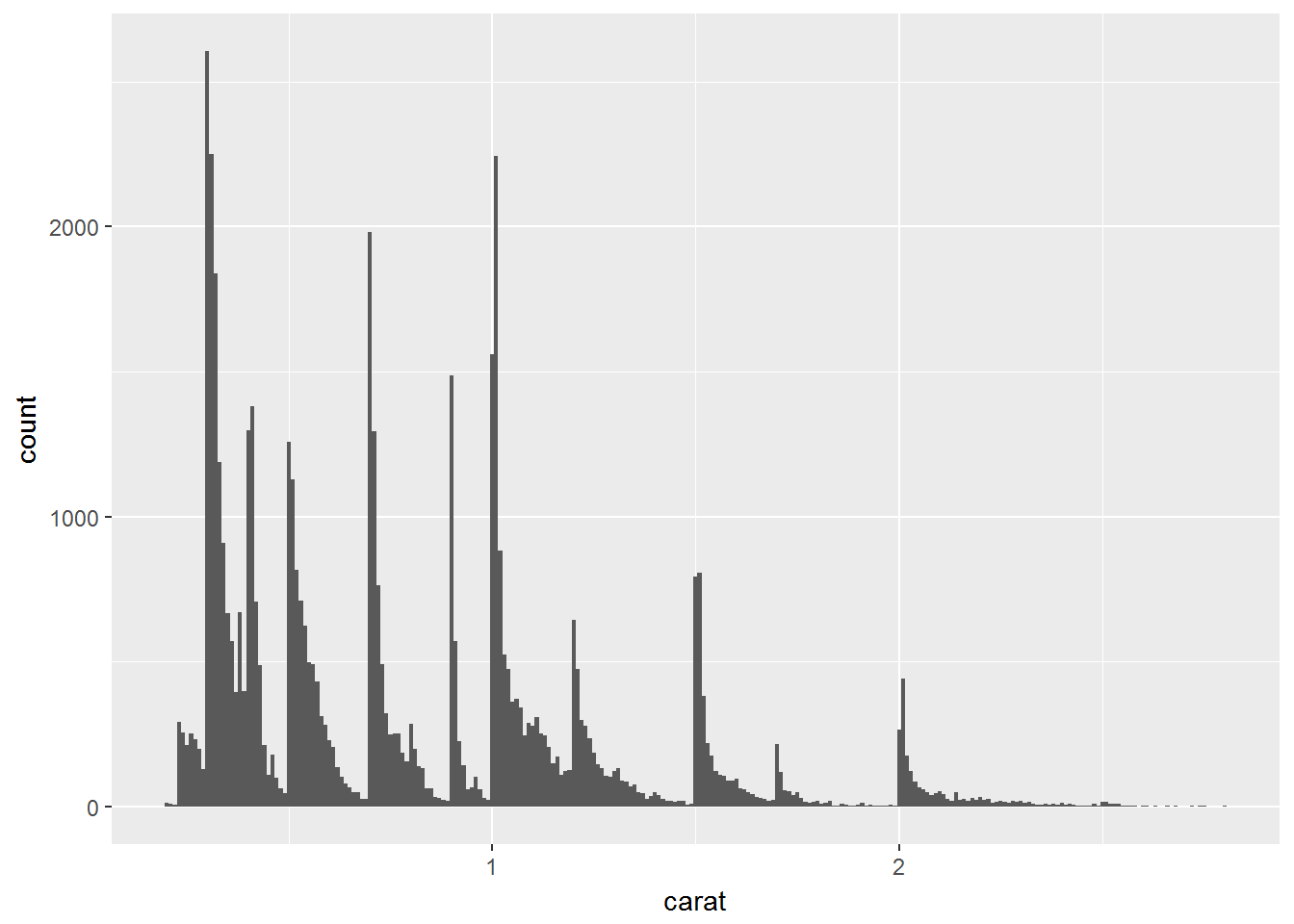
观察到了钻石有聚类现象,则对聚类提出问题:
- How are the observations within each cluster similar to each other?
- How are the observations in separate clusters different from each other?
- How can you explain or describe the clusters?
- Why might the appearance of clusters be misleading?
老忠实泉的喷发时间
ggplot(data = faithful, mapping = aes(x = eruptions)) +
  geom_histogram(binwidth = 0.25)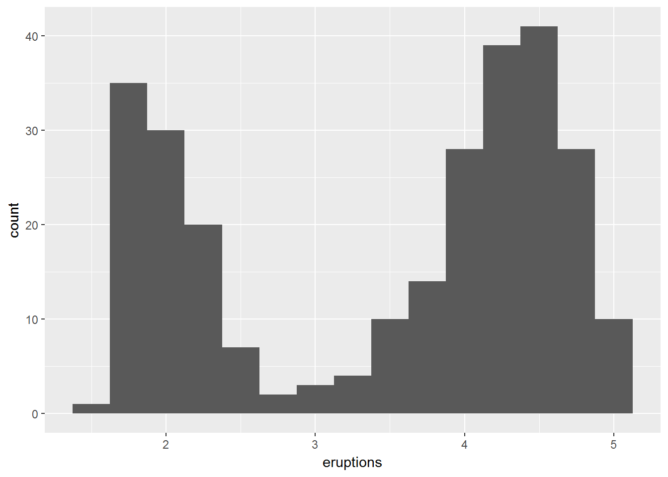
为什么老忠实泉有两个集中的喷发时间,中间却很少。
提出一些问题引导探索,比如,一些变量的分布是否能通过其他变量来解释。即变量之间的相互关系。
异常值
非典型值有两种情况:
- 错误数据;
- 蕴含重要新知识的数据;
当数据量很大时,离群点不容易被发现。
ggplot(diamonds) +
  geom_histogram(mapping = aes(x = y), binwidth = 0.5)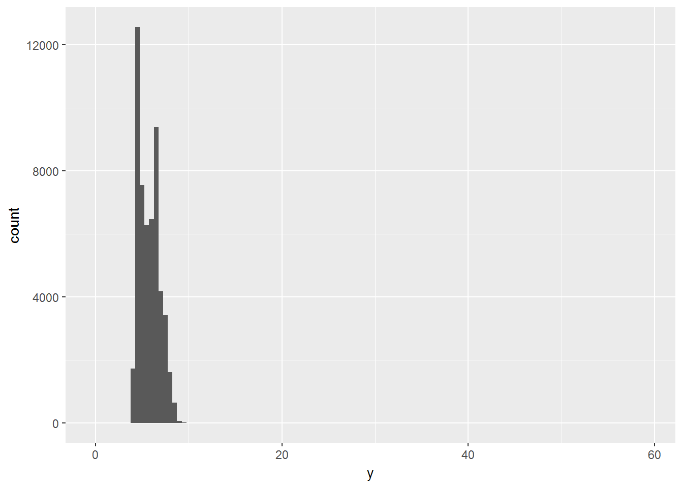
因为直方图被压缩,所以意识到有个很大的值。
为了发现缺失值,可以zoom in到小值的范围
ggplot(diamonds) +
  geom_histogram(mapping = aes(x = y), binwidth = 0.5) +
  coord_cartesian(ylim = c(0, 50))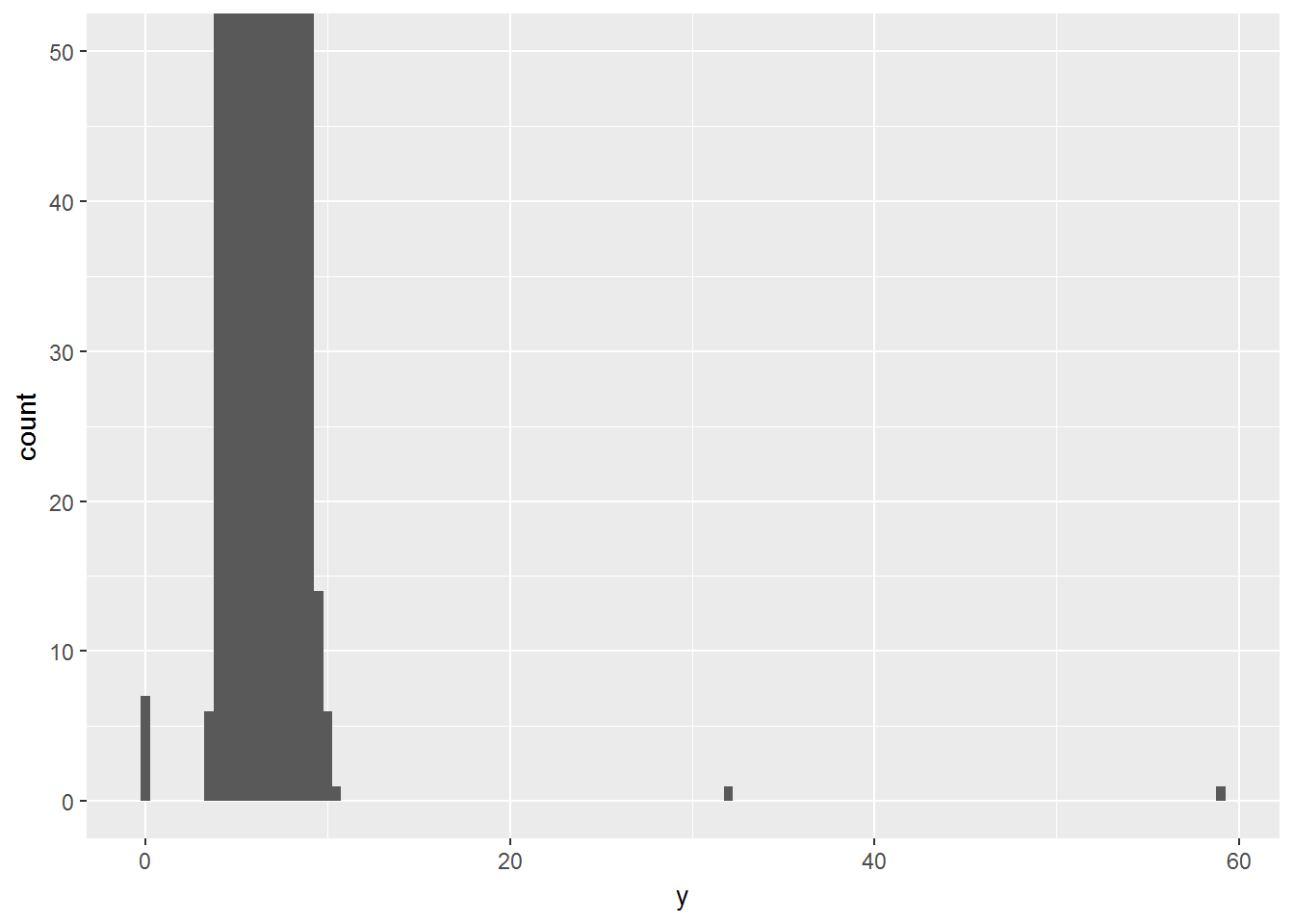
区别于xlim()和ylim(),这两个是将超出范围的样本扔掉
存在3个异常值,挑选出来
unusual <- diamonds %>%
  filter(y < 3 | y > 20) %>%
  select(price, x, y, z) %>%
  arrange(y)
unusual
## # A tibble: 9 x 4
## price x y z
## <int> <dbl> <dbl> <dbl>
## 1 5139 0 0 0
## 2 6381 0 0 0
## 3 12800 0 0 0
## 4 15686 0 0 0
## 5 18034 0 0 0
## 6 2130 0 0 0
## 7 2130 0 0 0
## 8 2075 5.15 31.8 5.12
## 9 12210 8.09 58.9 8.06发现这些异常数据都是有问题的。
不推荐不加考虑直接扔掉。因为一个观测存在一个值是异常值,不代表其他值也是异常值。直接丢掉会很可惜。
对于异常值,如果不知道为什么产生,可以将其替换为缺失值。
diamonds2 <- diamonds %>%
  mutate(y = ifelse(y < 3 | y > 20, NA, y))
缺失值
ggplot(data = diamonds2, mapping = aes(x = x, y = y)) +
  geom_point()
## Warning: Removed 9 rows containing missing values (geom_point).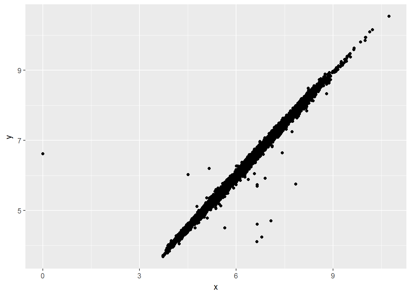
如果不想要提示,加上na.rm=T
为了探寻缺失值的模式,可以将缺失单列出一个变量
nycflights13::flights %>%
  mutate(
    cancelled = is.na(dep_time),
    sched_hour = sched_dep_time %/% 100,
    sched_min = sched_dep_time %% 100,
    sched_dep_time = sched_hour + sched_min / 60
  ) %>%
  ggplot(mapping = aes(sched_dep_time)) +
    geom_freqpoly(mapping = aes(colour = cancelled), binwidth = 1/4)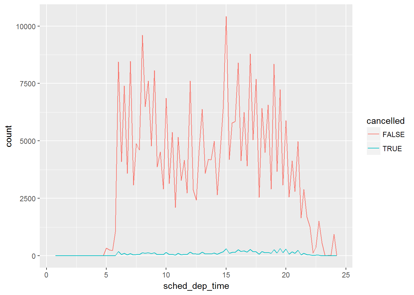
然而由于没有取消的航班远远多于取消的航班,所以看不出规律。
使用分面。
nycflights13::flights %>%
  mutate(
    cancelled = is.na(dep_time),
    sched_hour = sched_dep_time %/% 100,
    sched_min = sched_dep_time %% 100,
    sched_dep_time = sched_hour + sched_min / 60
  ) %>%
  ggplot(mapping = aes(sched_dep_time)) +
    geom_freqpoly(mapping = aes(colour = cancelled), binwidth = 1/4)+
    facet_wrap(~cancelled,nrow = 2,scales = "free_y")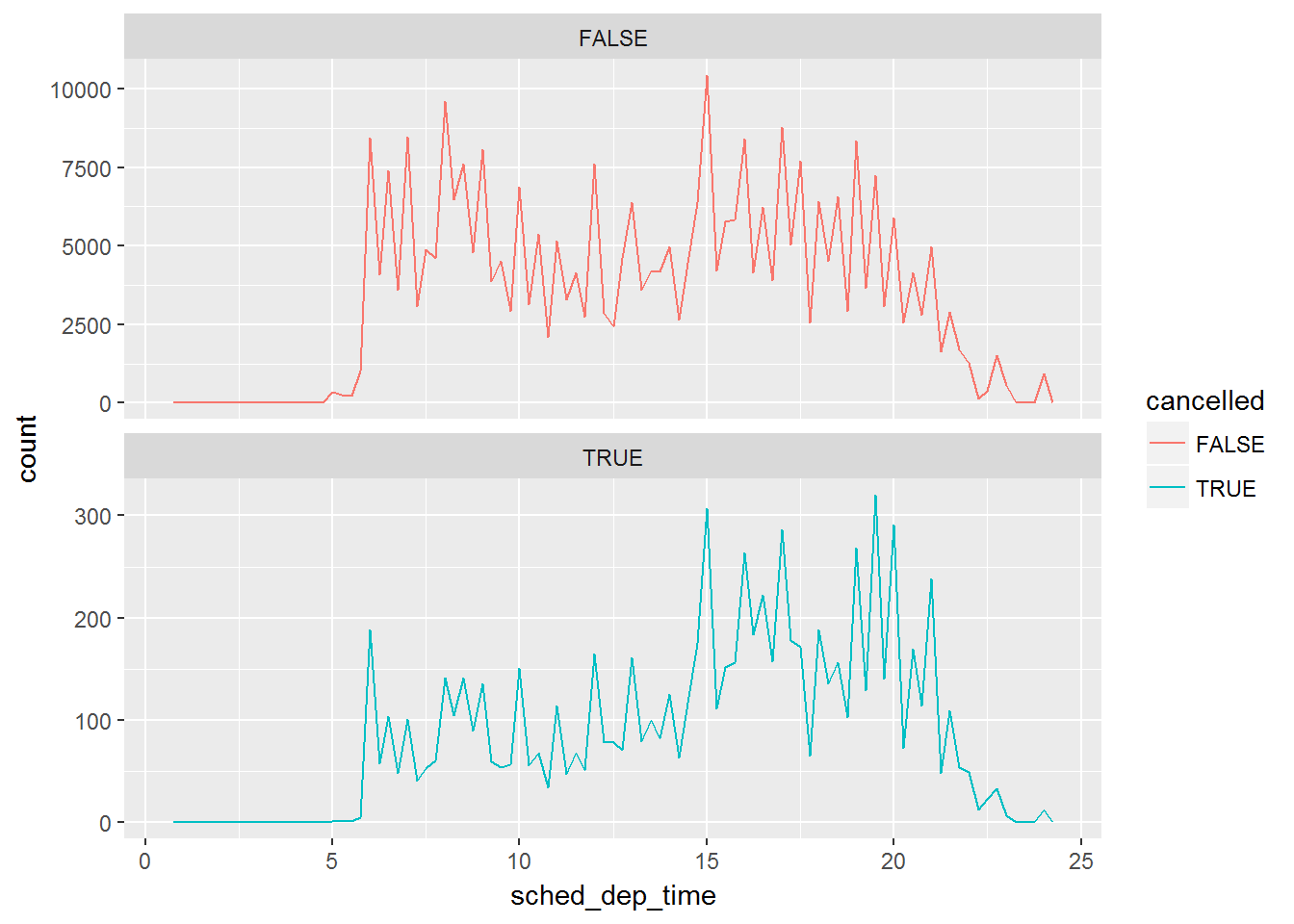
Covariation
多个变量之间的协变化关系
一个分类变量和一个连续变量
geom_freqpoly()不太容易比较,因为高度是由count给出的
ggplot(data = diamonds, mapping = aes(x = price)) +
  geom_freqpoly(mapping = aes(colour = cut), binwidth = 500)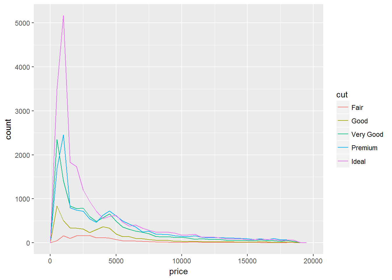
因为每组中样本量相差很大,所以分布的差别不容易看出来。
ggplot(diamonds) +
  geom_bar(mapping = aes(x = cut))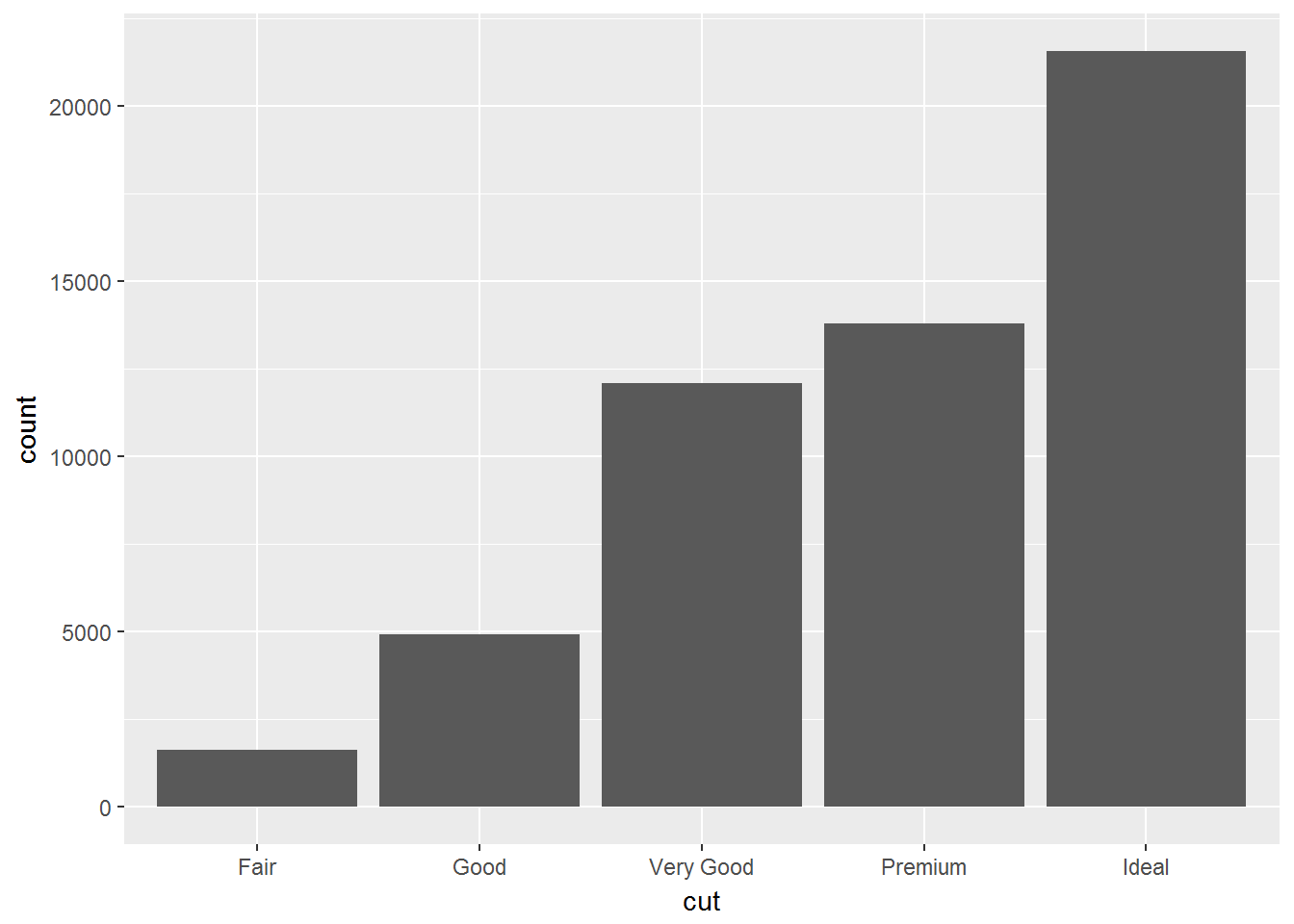
为了消除量的差别,y坐标需要调整,改成density,是count的标准化结果
ggplot(data = diamonds, mapping = aes(x = price, y = ..density..)) +
  geom_freqpoly(mapping = aes(colour = cut), binwidth = 500)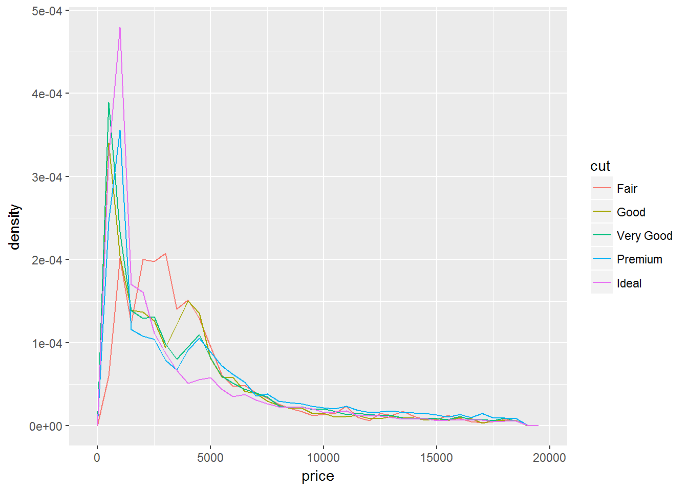
除了直方图外,还可以用箱线图看分布,箱体内(IQR)是25%~75%,离群点是超过1.5个IQR
ggplot(data = diamonds, mapping = aes(x = cut, y = price)) +
  geom_boxplot()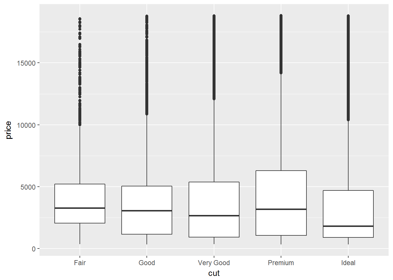
当分类变量是无序的时,可以考虑重新排序
ggplot(data = mpg, mapping = aes(x = class, y = hwy)) +
  geom_boxplot()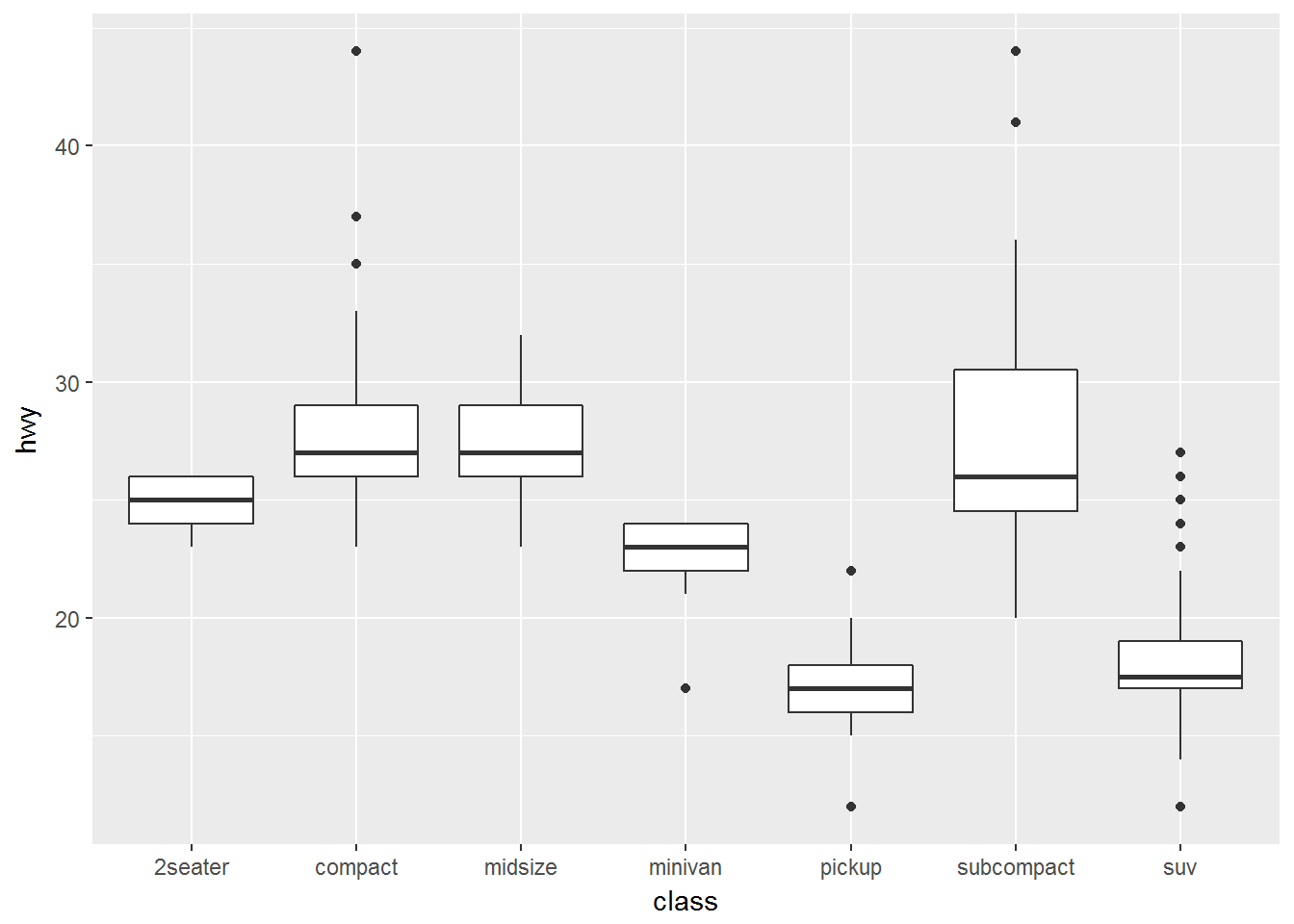
ggplot(data = mpg) +
  geom_boxplot(mapping = aes(x = reorder(class, hwy, FUN = median), y = hwy))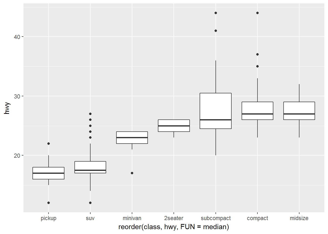
如果变量名较长,可以翻转xy坐标
ggplot(data = mpg) +
  geom_boxplot(mapping = aes(x = reorder(class, hwy, FUN = median), y = hwy)) +
  coord_flip()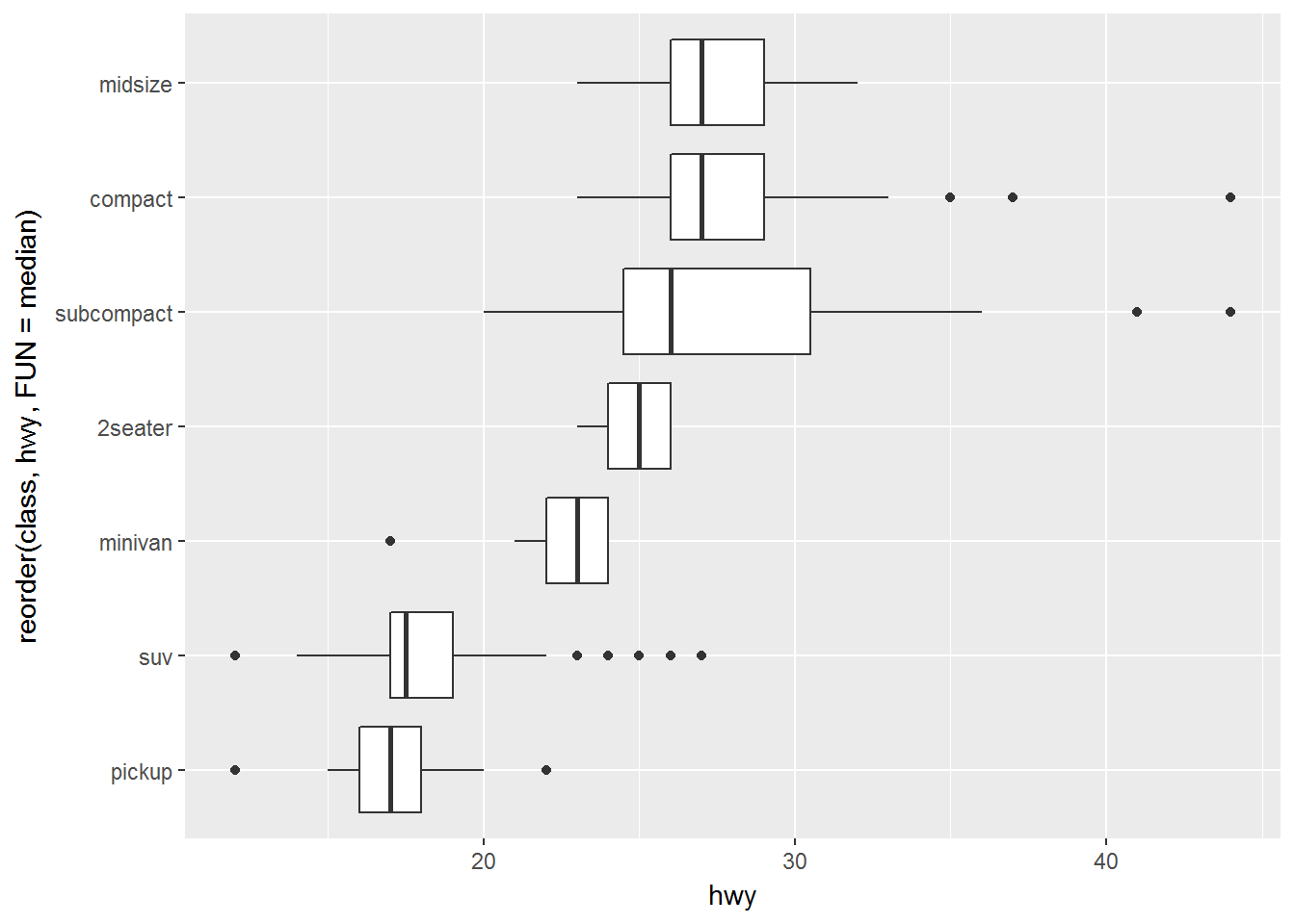
两个分类变量
ggplot(data = diamonds) +
  geom_count(mapping = aes(x = cut, y = color))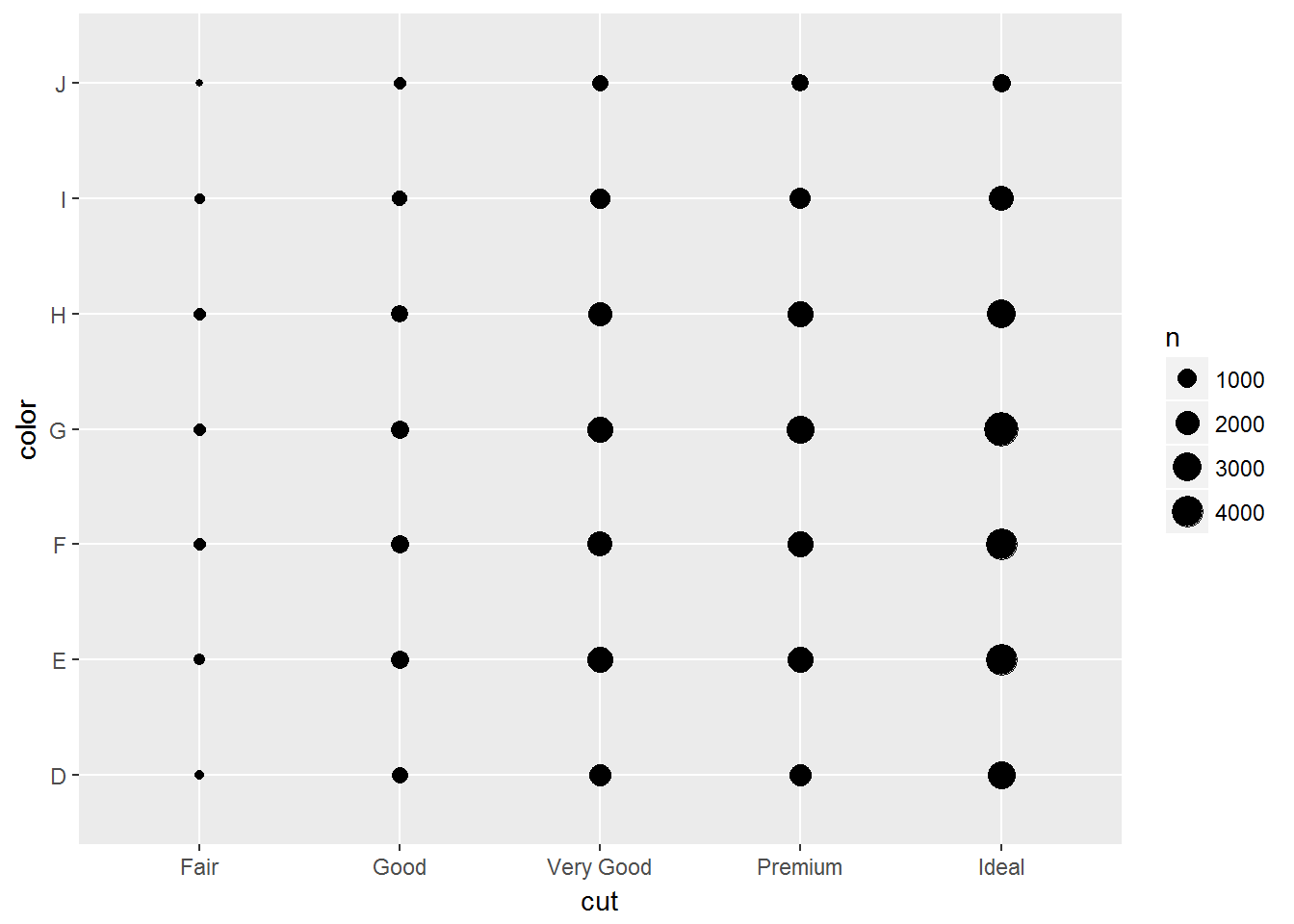
相当于列联表的可视化
table(diamonds$color,diamonds$cut)##
## Fair Good Very Good Premium Ideal
## D 163 662 1513 1603 2834
## E 224 933 2400 2337 3903
## F 312 909 2164 2331 3826
## G 314 871 2299 2924 4884
## H 303 702 1824 2360 3115
## I 175 522 1204 1428 2093
## J 119 307 678 808 896可以用瓦块图
diamonds %>%
  count(color, cut)
## # A tibble: 35 x 3
## color cut n
## <ord> <ord> <int>
## 1 D Fair 163
## 2 D Good 662
## 3 D Very Good 1513
## 4 D Premium 1603
## 5 D Ideal 2834
## 6 E Fair 224
## 7 E Good 933
## 8 E Very Good 2400
## 9 E Premium 2337
## 10 E Ideal 3903
## # ... with 25 more rowsdiamonds %>%
count(color, cut) %>%
ggplot(mapping = aes(x = color, y = cut)) +
geom_tile(mapping = aes(fill = n))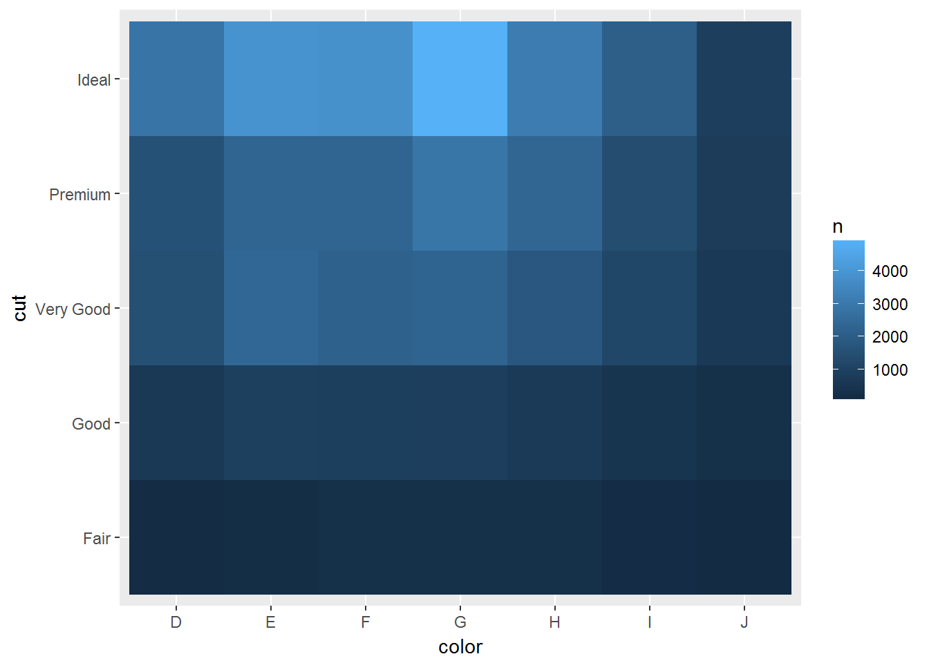
两个连续变量
使用散点图
ggplot(data = diamonds) +
  geom_point(mapping = aes(x = carat, y = price))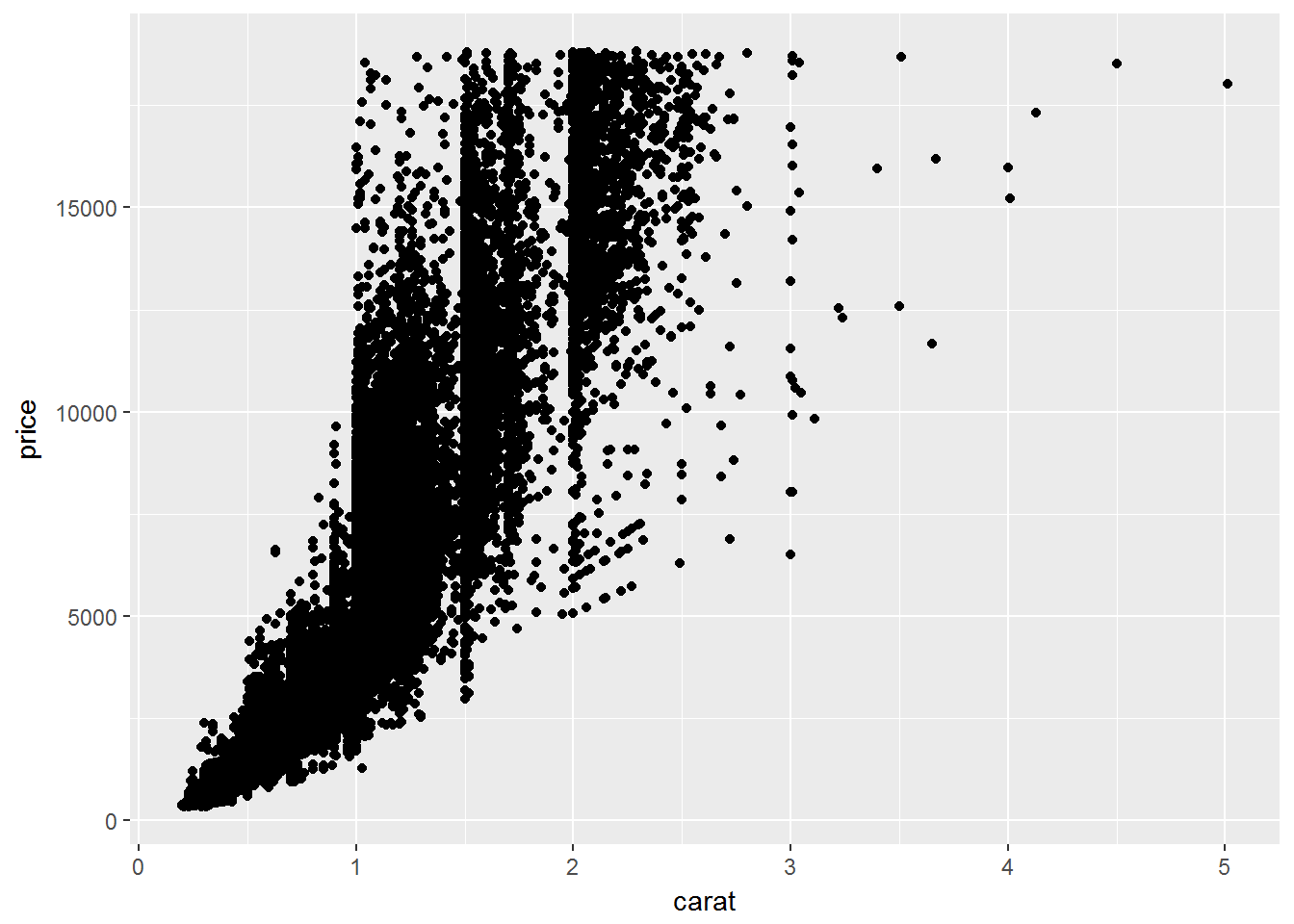
如果点很多的话,散点图就看不清楚,可以加上透明度
ggplot(data = diamonds) +
  geom_point(mapping = aes(x = carat, y = price), alpha = 1 / 100)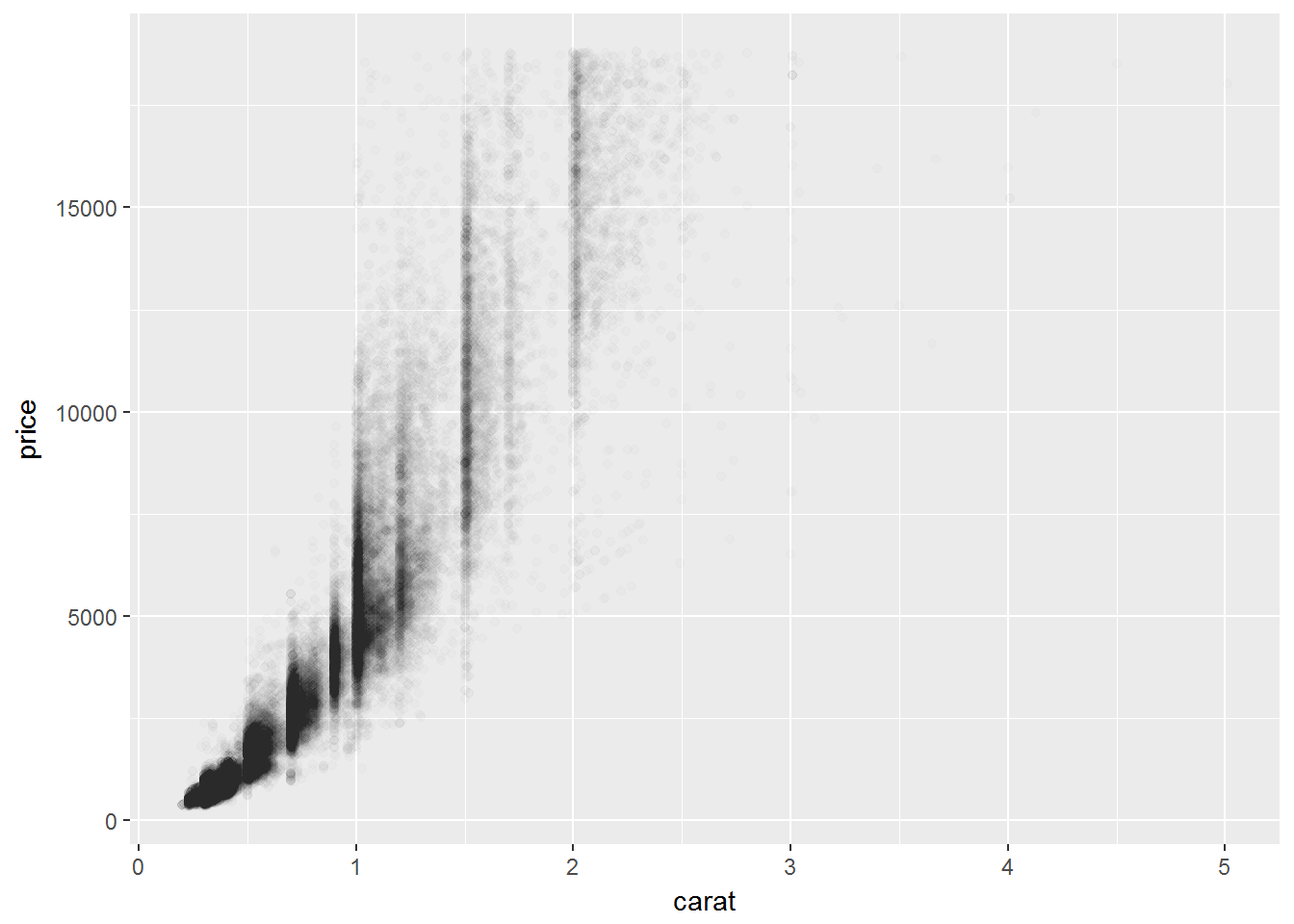
也可以使用二维分箱
smaller <- diamonds %>%
  filter(carat < 3)
ggplot(data = smaller) +
  geom_bin2d(mapping = aes(x = carat, y = price))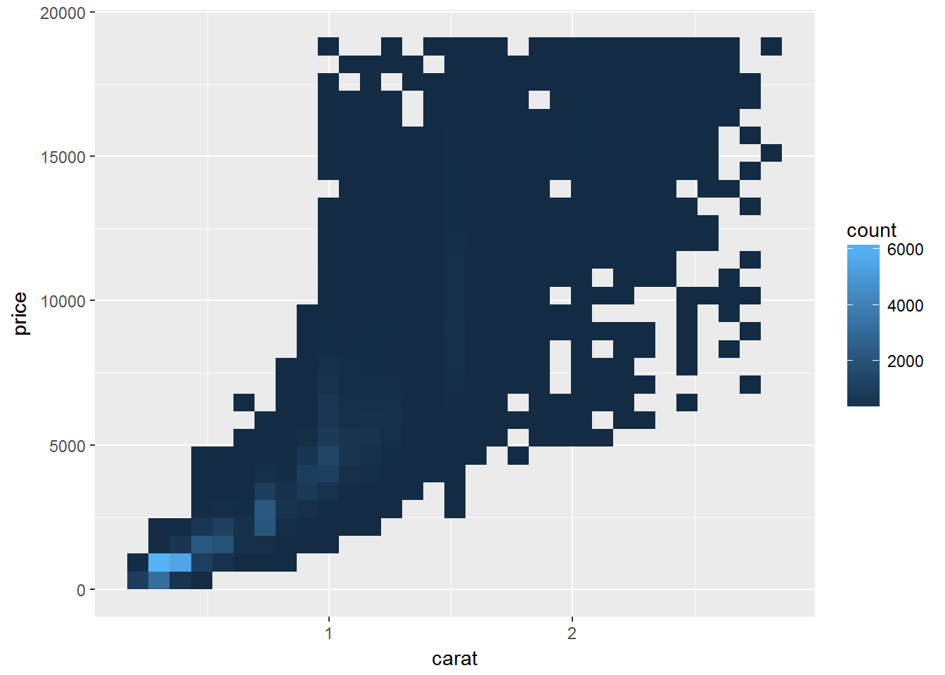
# install.packages("hexbin")
ggplot(data = smaller) +
  geom_hex(mapping = aes(x = carat, y = price))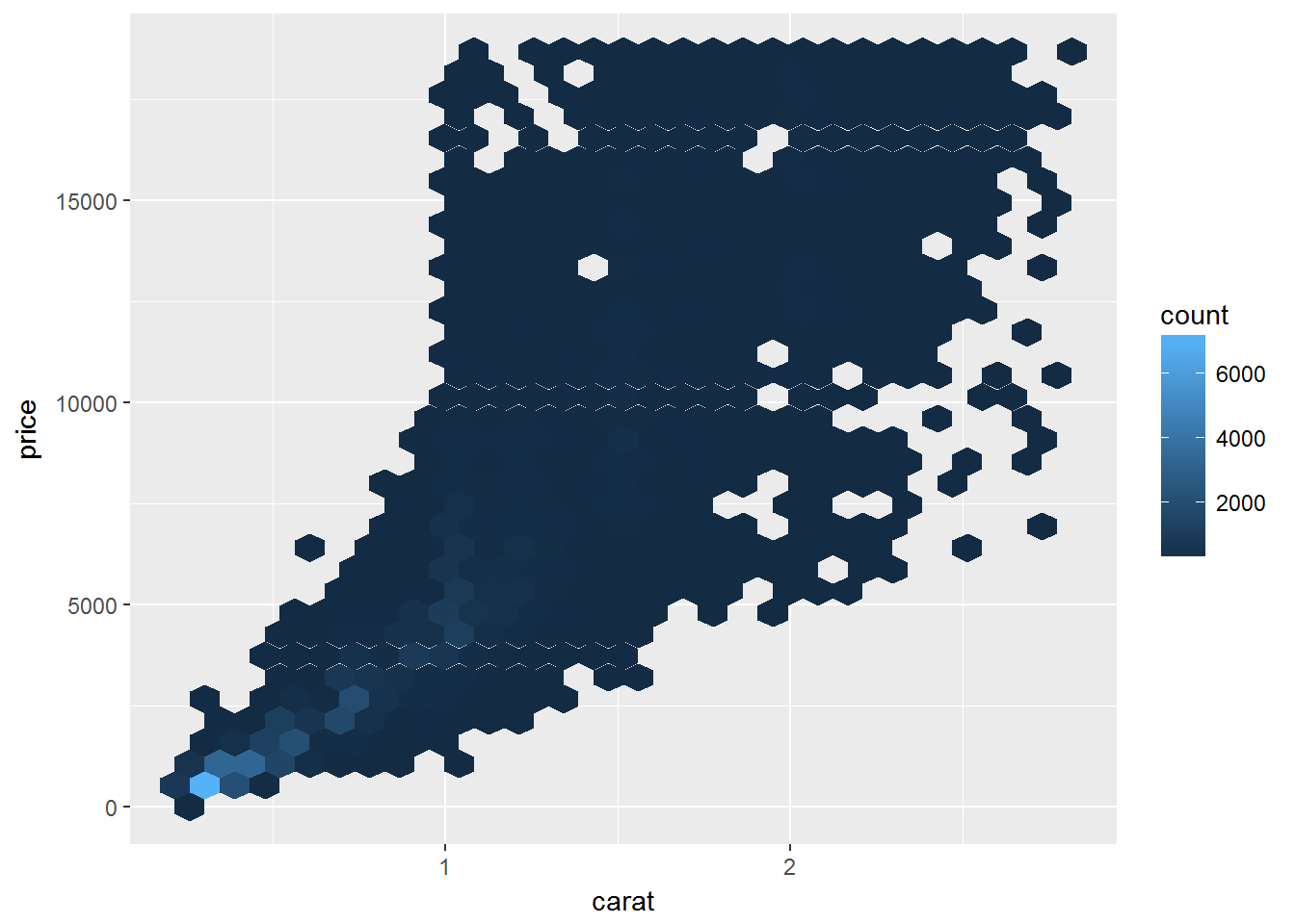
也可以选择在一个维度上装箱,则变成了分类和连续变量问题
使用group来分组
ggplot(data = smaller, mapping = aes(x = carat, y = price)) +
  geom_boxplot(mapping = aes(group = cut_width(carat, 0.1)))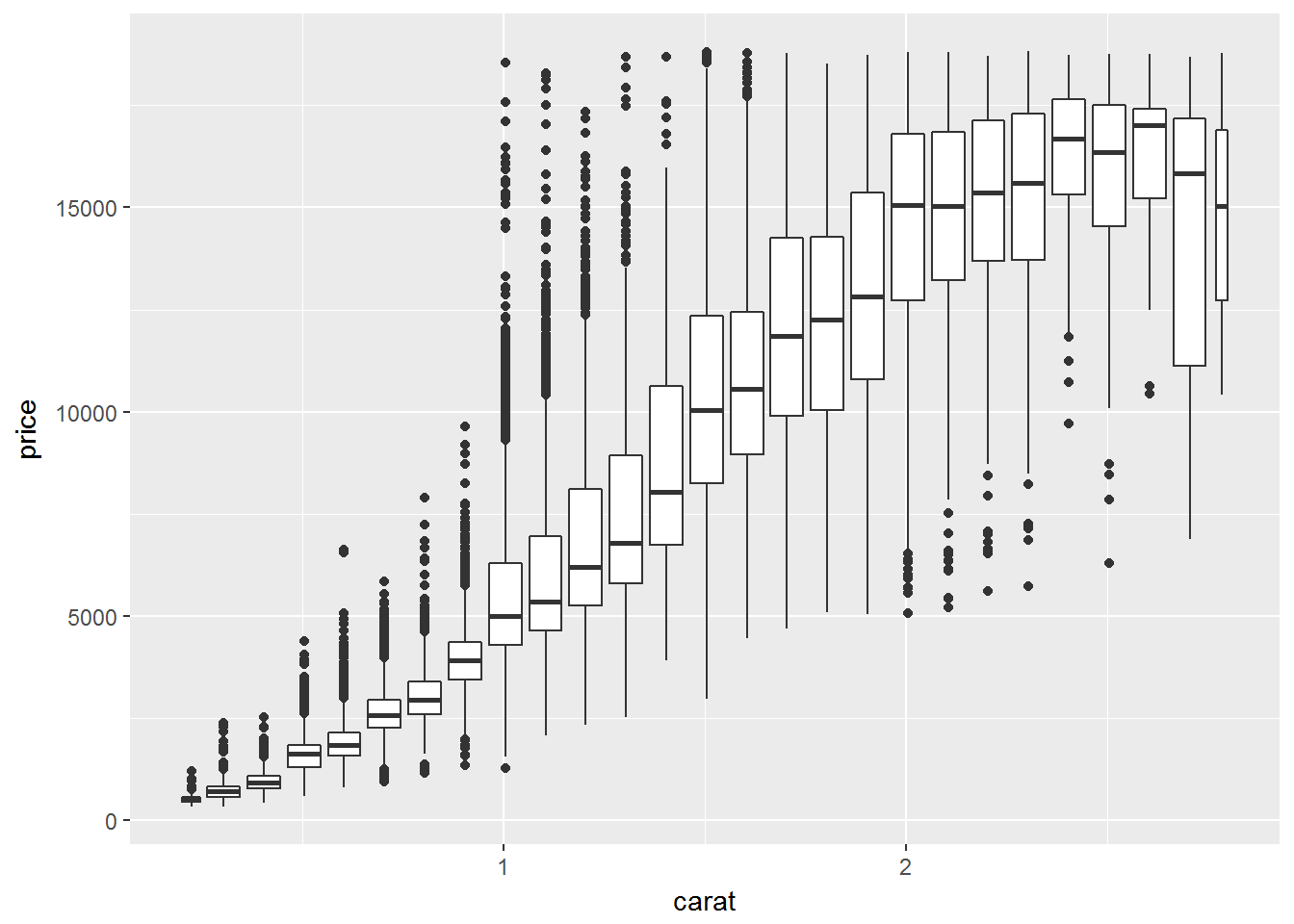
但cut_width()每一个箱体都是等宽的,所以不能反映该分组中样本数量,可以通过设置
ggplot(data = smaller, mapping = aes(x = carat, y = price)) +
  geom_boxplot(mapping = aes(group = cut_width(carat, 0.1)),varwidth = T)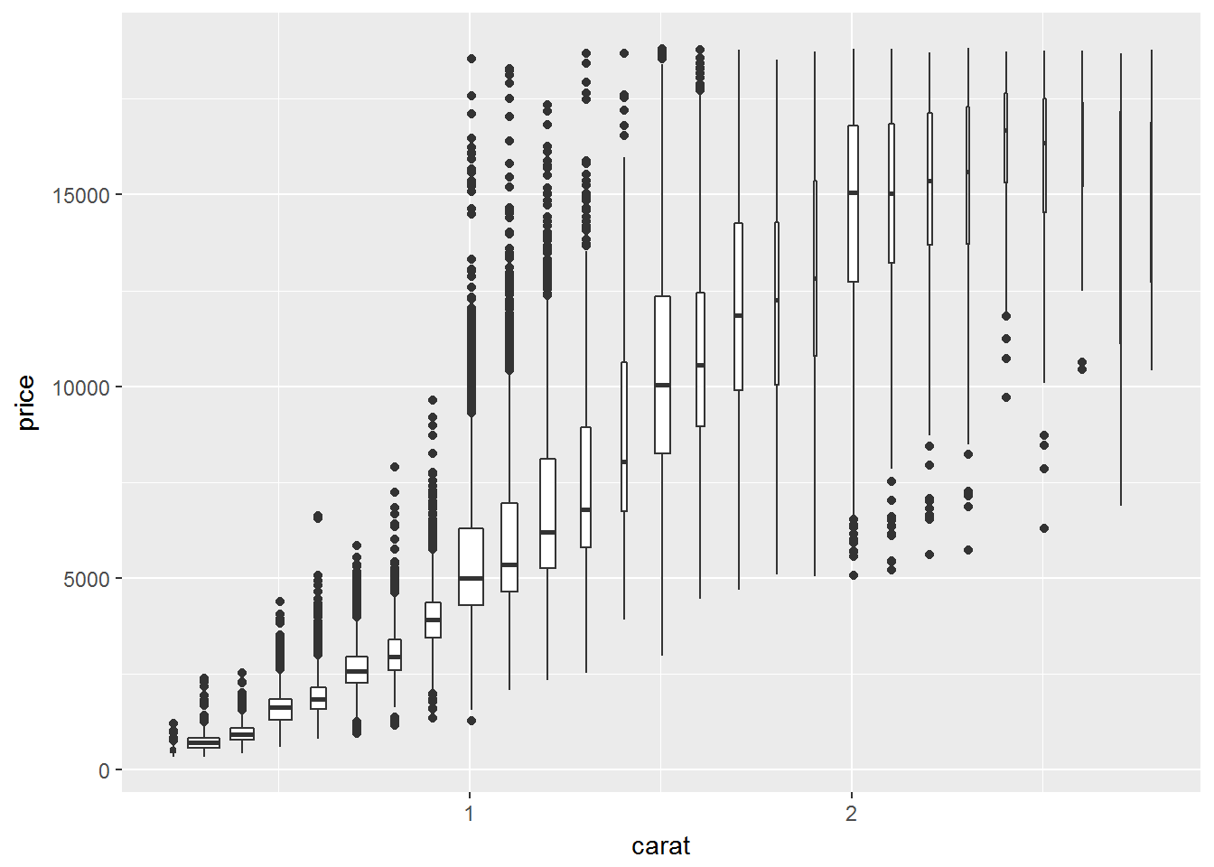
模式和模型
关于模式可以提出的问题:
- Could this pattern be due to coincidence (i.e. random chance)?
- How can you describe the relationship implied by the pattern?
- How strong is the relationship implied by the pattern?
- What other variables might affect the relationship?
- Does the relationship change if you look at individual subgroups of the data?
ggplot(data = faithful) +
  geom_point(mapping = aes(x = eruptions, y = waiting))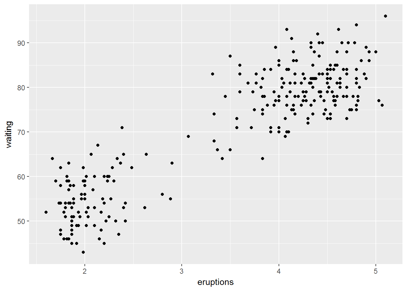
模式是很重要的,因为利于发现相关关系。
如果说variation是增加了不确定性,covariation则是减少了不确定性。
模型是一种提取模式的方法。
钻石问题中,首先移除carat对price的影响
mod <- lm(log(price) ~ log(carat), data = diamonds)
diamonds2 <- diamonds %>%
  add_residuals(mod) %>%
  mutate(resid = exp(resid))

ggplot(data = diamonds2) +
  geom_point(mapping = aes(x = carat, y = resid))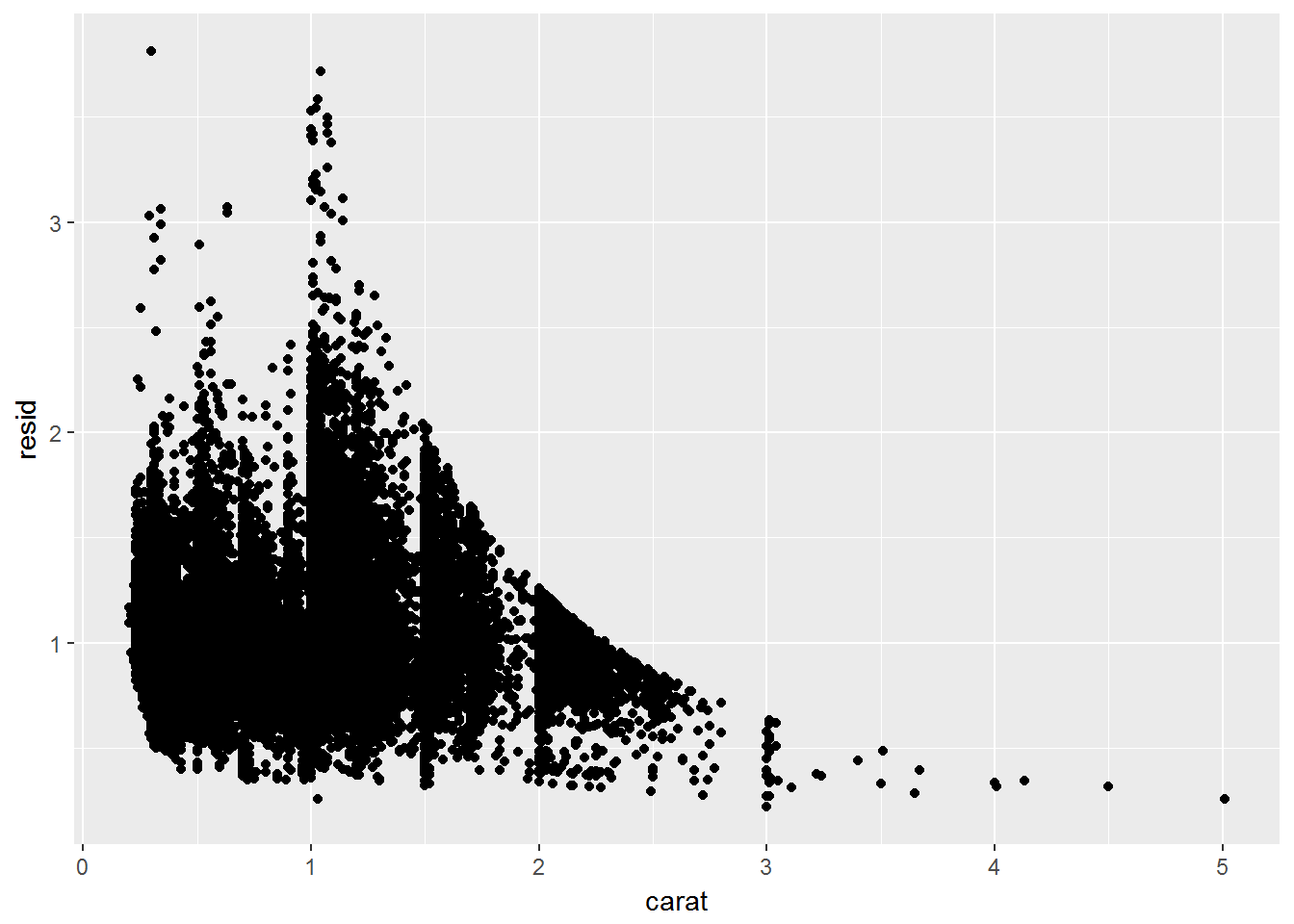
当移除了carat对price的影响后,就可以看cut对price的影响了
ggplot(data = diamonds2) +
  geom_boxplot(mapping = aes(x = cut, y = resid))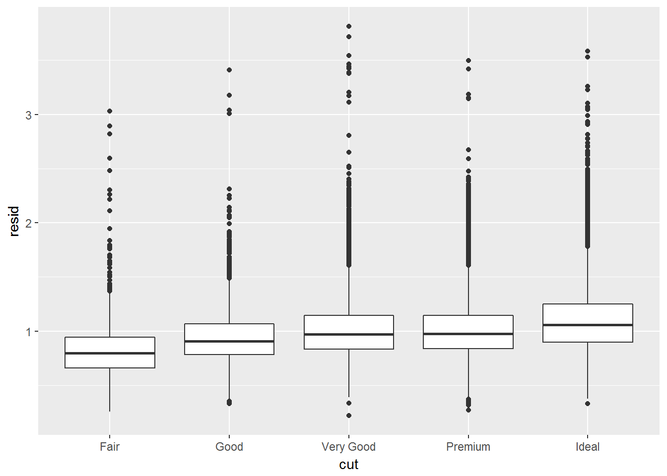
当移除了克拉因素后,切割越好价格越高。
Project式工作流
- C+S+F10重启Rstudio
- C+S+S运行当前脚本
对于路径来说:
- 最好使用斜杠而不是反斜杠;
- 不要使用绝对路径,因为别人的路径和你的不一样;
Project工作流
- Create an RStudio project for each data analysis project.
- Keep data files there; we’ll talk about loading them into R in data import.
- Keep scripts there; edit them, run them in bits or as a whole.
- Save your outputs (plots and cleaned data) there.
- Only ever use relative paths, not absolute paths.