使用dplyr包进行数据变形
library(tidyverse)## Warning: 程辑包'tidyverse'是用R版本3.5.1 来建造的## -- Attaching packages -------------------------------------------------------- tidyverse 1.2.1 --## √ ggplot2 2.2.1 √ purrr 0.2.5
## √ tibble 1.4.2 √ dplyr 0.7.6
## √ tidyr 0.8.1 √ stringr 1.3.1
## √ readr 1.1.1 √ forcats 0.3.0## Warning: 程辑包'tidyr'是用R版本3.5.1 来建造的## Warning: 程辑包'readr'是用R版本3.5.1 来建造的## Warning: 程辑包'forcats'是用R版本3.5.1 来建造的## -- Conflicts ----------------------------------------------------------- tidyverse_conflicts() --
## x dplyr::filter() masks stats::filter()
## x dplyr::lag() masks stats::lag()library(nycflights13)## Warning: 程辑包'nycflights13'是用R版本3.5.1 来建造的tibble是一种基于data.frame的数据类型,为了更好地适应于tidyverse包。
几种数据类型的简写:
- int
- dbl
- chr
- dttm date-times
- lgl logical
- fctr factor
- date
dplyr中的重要函数:
- filter() 根据观测值选择观测;
- arrange() 行重新排序;
- select() 根据变量名选择变量;
- mutate() 根据已存在变量和函数创造新变量;
- summarise() 产生汇总值
- group_by() 分组运行
语法:
- 第一个参数是df;
- 之后的参数描述变换,使用不带引号的变量名;
- 结果是新的df;
案例数据 flights
str(flights)## Classes 'tbl_df', 'tbl' and 'data.frame': 336776 obs. of 19 variables:
## $ year : int 2013 2013 2013 2013 2013 2013 2013 2013 2013 2013 ...
## $ month : int 1 1 1 1 1 1 1 1 1 1 ...
## $ day : int 1 1 1 1 1 1 1 1 1 1 ...
## $ dep_time : int 517 533 542 544 554 554 555 557 557 558 ...
## $ sched_dep_time: int 515 529 540 545 600 558 600 600 600 600 ...
## $ dep_delay : num 2 4 2 -1 -6 -4 -5 -3 -3 -2 ...
## $ arr_time : int 830 850 923 1004 812 740 913 709 838 753 ...
## $ sched_arr_time: int 819 830 850 1022 837 728 854 723 846 745 ...
## $ arr_delay : num 11 20 33 -18 -25 12 19 -14 -8 8 ...
## $ carrier : chr "UA" "UA" "AA" "B6" ...
## $ flight : int 1545 1714 1141 725 461 1696 507 5708 79 301 ...
## $ tailnum : chr "N14228" "N24211" "N619AA" "N804JB" ...
## $ origin : chr "EWR" "LGA" "JFK" "JFK" ...
## $ dest : chr "IAH" "IAH" "MIA" "BQN" ...
## $ air_time : num 227 227 160 183 116 150 158 53 140 138 ...
## $ distance : num 1400 1416 1089 1576 762 ...
## $ hour : num 5 5 5 5 6 5 6 6 6 6 ...
## $ minute : num 15 29 40 45 0 58 0 0 0 0 ...
## $ time_hour : POSIXct, format: "2013-01-01 05:00:00" "2013-01-01 05:00:00" ...filter()
filter(flights, month == 1, day ==1)## # A tibble: 842 x 19
## year month day dep_time sched_dep_time dep_delay arr_time
## <int> <int> <int> <int> <int> <dbl> <int>
## 1 2013 1 1 517 515 2 830
## 2 2013 1 1 533 529 4 850
## 3 2013 1 1 542 540 2 923
## 4 2013 1 1 544 545 -1 1004
## 5 2013 1 1 554 600 -6 812
## 6 2013 1 1 554 558 -4 740
## 7 2013 1 1 555 600 -5 913
## 8 2013 1 1 557 600 -3 709
## 9 2013 1 1 557 600 -3 838
## 10 2013 1 1 558 600 -2 753
## # ... with 832 more rows, and 12 more variables: sched_arr_time <int>,
## # arr_delay <dbl>, carrier <chr>, flight <int>, tailnum <chr>,
## # origin <chr>, dest <chr>, air_time <dbl>, distance <dbl>, hour <dbl>,
## # minute <dbl>, time_hour <dttm>tidyverse的函数不修改原来的df.
- 比较运算符 > >= < <= != ==
- 逻辑运算符 & | |!
- %in%
nov_dec <- filter(flights, month %in% c(11,12))
dim(nov_dec)
## [1] 55403 19注意:
- 在这里不要使用&&和||
- NA是传染性的
arrange()
arrange(flights, year, month, day)## # A tibble: 336,776 x 19
## year month day dep_time sched_dep_time dep_delay arr_time
## <int> <int> <int> <int> <int> <dbl> <int>
## 1 2013 1 1 517 515 2 830
## 2 2013 1 1 533 529 4 850
## 3 2013 1 1 542 540 2 923
## 4 2013 1 1 544 545 -1 1004
## 5 2013 1 1 554 600 -6 812
## 6 2013 1 1 554 558 -4 740
## 7 2013 1 1 555 600 -5 913
## 8 2013 1 1 557 600 -3 709
## 9 2013 1 1 557 600 -3 838
## 10 2013 1 1 558 600 -2 753
## # ... with 336,766 more rows, and 12 more variables: sched_arr_time <int>,
## # arr_delay <dbl>, carrier <chr>, flight <int>, tailnum <chr>,
## # origin <chr>, dest <chr>, air_time <dbl>, distance <dbl>, hour <dbl>,
## # minute <dbl>, time_hour <dttm>desc()函数用来降序排列
arrange(flights, desc(dep_delay))## # A tibble: 336,776 x 19
## year month day dep_time sched_dep_time dep_delay arr_time
## <int> <int> <int> <int> <int> <dbl> <int>
## 1 2013 1 9 641 900 1301 1242
## 2 2013 6 15 1432 1935 1137 1607
## 3 2013 1 10 1121 1635 1126 1239
## 4 2013 9 20 1139 1845 1014 1457
## 5 2013 7 22 845 1600 1005 1044
## 6 2013 4 10 1100 1900 960 1342
## 7 2013 3 17 2321 810 911 135
## 8 2013 6 27 959 1900 899 1236
## 9 2013 7 22 2257 759 898 121
## 10 2013 12 5 756 1700 896 1058
## # ... with 336,766 more rows, and 12 more variables: sched_arr_time <int>,
## # arr_delay <dbl>, carrier <chr>, flight <int>, tailnum <chr>,
## # origin <chr>, dest <chr>, air_time <dbl>, distance <dbl>, hour <dbl>,
## # minute <dbl>, time_hour <dttm>NA值通常被排序到最后
select()
select(flights, year, month, day)## # A tibble: 336,776 x 3
## year month day
## <int> <int> <int>
## 1 2013 1 1
## 2 2013 1 1
## 3 2013 1 1
## 4 2013 1 1
## 5 2013 1 1
## 6 2013 1 1
## 7 2013 1 1
## 8 2013 1 1
## 9 2013 1 1
## 10 2013 1 1
## # ... with 336,766 more rowsselect(flights, year:day)## # A tibble: 336,776 x 3
## year month day
## <int> <int> <int>
## 1 2013 1 1
## 2 2013 1 1
## 3 2013 1 1
## 4 2013 1 1
## 5 2013 1 1
## 6 2013 1 1
## 7 2013 1 1
## 8 2013 1 1
## 9 2013 1 1
## 10 2013 1 1
## # ... with 336,766 more rowsselect(flights, -(year:day))## # A tibble: 336,776 x 16
## dep_time sched_dep_time dep_delay arr_time sched_arr_time arr_delay
## <int> <int> <dbl> <int> <int> <dbl>
## 1 517 515 2 830 819 11
## 2 533 529 4 850 830 20
## 3 542 540 2 923 850 33
## 4 544 545 -1 1004 1022 -18
## 5 554 600 -6 812 837 -25
## 6 554 558 -4 740 728 12
## 7 555 600 -5 913 854 19
## 8 557 600 -3 709 723 -14
## 9 557 600 -3 838 846 -8
## 10 558 600 -2 753 745 8
## # ... with 336,766 more rows, and 10 more variables: carrier <chr>,
## # flight <int>, tailnum <chr>, origin <chr>, dest <chr>, air_time <dbl>,
## # distance <dbl>, hour <dbl>, minute <dbl>, time_hour <dttm>helper函数
select()可以和一些helper函数一起使用:
- start_with(“abc”)
- ends_with(“xyz”)
- contains(“ijk”)
- mathches(“(.)\1”)
- num_range(“x”,1:3)
df <- data.frame(x1=1:10,x2=letters[1:10],x3=LETTERS[1:10],x4=10:1)
select(df,num_range("x",1:3))
## x1 x2 x3
## 1 1 a A
## 2 2 b B
## 3 3 c C
## 4 4 d D
## 5 5 e E
## 6 6 f F
## 7 7 g G
## 8 8 h H
## 9 9 i I
## 10 10 j J如果要更名变量,使用rename()
names(flights)## [1] "year" "month" "day" "dep_time"
## [5] "sched_dep_time" "dep_delay" "arr_time" "sched_arr_time"
## [9] "arr_delay" "carrier" "flight" "tailnum"
## [13] "origin" "dest" "air_time" "distance"
## [17] "hour" "minute" "time_hour"df <- rename(flights,tail_num = tailnum)
names(df)## [1] "year" "month" "day" "dep_time"
## [5] "sched_dep_time" "dep_delay" "arr_time" "sched_arr_time"
## [9] "arr_delay" "carrier" "flight" "tail_num"
## [13] "origin" "dest" "air_time" "distance"
## [17] "hour" "minute" "time_hour"将重要的变量排在前面
select(flights, time_hour, air_time, everything())## # A tibble: 336,776 x 19
## time_hour air_time year month day dep_time sched_dep_time
## <dttm> <dbl> <int> <int> <int> <int> <int>
## 1 2013-01-01 05:00:00 227 2013 1 1 517 515
## 2 2013-01-01 05:00:00 227 2013 1 1 533 529
## 3 2013-01-01 05:00:00 160 2013 1 1 542 540
## 4 2013-01-01 05:00:00 183 2013 1 1 544 545
## 5 2013-01-01 06:00:00 116 2013 1 1 554 600
## 6 2013-01-01 05:00:00 150 2013 1 1 554 558
## 7 2013-01-01 06:00:00 158 2013 1 1 555 600
## 8 2013-01-01 06:00:00 53 2013 1 1 557 600
## 9 2013-01-01 06:00:00 140 2013 1 1 557 600
## 10 2013-01-01 06:00:00 138 2013 1 1 558 600
## # ... with 336,766 more rows, and 12 more variables: dep_delay <dbl>,
## # arr_time <int>, sched_arr_time <int>, arr_delay <dbl>, carrier <chr>,
## # flight <int>, tailnum <chr>, origin <chr>, dest <chr>, distance <dbl>,
## # hour <dbl>, minute <dbl>mutate()
flights_sml <- select(flights,
  year:day,
  ends_with("delay"),
  distance,
  air_time
)
mutate(flights_sml,
  gain = dep_delay - arr_delay,
  speed = distance / air_time * 60
) %>% names()
## [1] "year" "month" "day" "dep_delay" "arr_delay" "distance"
## [7] "air_time" "gain" "speed"可以立即使用刚刚创建的变量
mutate(flights_sml,
  gain = dep_delay - arr_delay,
  hours = air_time / 60,
  gain_per_hour = gain / hours
) %>% names()
## [1] "year" "month" "day" "dep_delay"
## [5] "arr_delay" "distance" "air_time" "gain"
## [9] "hours" "gain_per_hour"如果只想保留新创建的变量,使用transmute()
transmute(flights,
  gain = dep_delay - arr_delay,
  hours = air_time / 60,
  gain_per_hour = gain / hours
)
## # A tibble: 336,776 x 3
## gain hours gain_per_hour
## <dbl> <dbl> <dbl>
## 1 -9 3.78 -2.38
## 2 -16 3.78 -4.23
## 3 -31 2.67 -11.6
## 4 17 3.05 5.57
## 5 19 1.93 9.83
## 6 -16 2.5 -6.4
## 7 -24 2.63 -9.11
## 8 11 0.883 12.5
## 9 5 2.33 2.14
## 10 -10 2.3 -4.35
## # ... with 336,766 more rows偏移(offset)函数
- lead
- lag
x <- 1:10
lead(x)
## [1] 2 3 4 5 6 7 8 9 10 NAlag(x)## [1] NA 1 2 3 4 5 6 7 8 9累积函数
- cumsum()
- cumprod()
- cummin()
- cummax()
summaries()
将数据框压缩到一行
summarise(flights, delay = mean(dep_delay, na.rm = TRUE))## # A tibble: 1 x 1
## delay
## <dbl>
## 1 12.6与group_by一起用
by_day <- group_by(flights, year, month, day)
summarise(by_day, delay = mean(dep_delay, na.rm = TRUE))
## # A tibble: 365 x 4
## # Groups: year, month [?]
## year month day delay
## <int> <int> <int> <dbl>
## 1 2013 1 1 11.5
## 2 2013 1 2 13.9
## 3 2013 1 3 11.0
## 4 2013 1 4 8.95
## 5 2013 1 5 5.73
## 6 2013 1 6 7.15
## 7 2013 1 7 5.42
## 8 2013 1 8 2.55
## 9 2013 1 9 2.28
## 10 2013 1 10 2.84
## # ... with 355 more rows对比plyr包,ddply的分而治之的思维更强,dplyr包group_by的易理解性更强。
ddply(flights,.variables = c("year","month","day"),summarise,delay=mean(dep_delay, na.rm = T))管道
by_dest <- group_by(flights, dest)
delay <- summarise(by_dest,
  count = n(),
  dist = mean(distance, na.rm = TRUE),
  delay = mean(arr_delay, na.rm = TRUE)
)
delay <- filter(delay, count > 20, dest != "HNL")
delay
## # A tibble: 96 x 4
## dest count dist delay
## <chr> <int> <dbl> <dbl>
## 1 ABQ 254 1826 4.38
## 2 ACK 265 199 4.85
## 3 ALB 439 143 14.4
## 4 ATL 17215 757. 11.3
## 5 AUS 2439 1514. 6.02
## 6 AVL 275 584. 8.00
## 7 BDL 443 116 7.05
## 8 BGR 375 378 8.03
## 9 BHM 297 866. 16.9
## 10 BNA 6333 758. 11.8
## # ... with 86 more rowsggplot(data = delay, mapping = aes(x = dist, y = delay)) +
geom_point(aes(size = count), alpha = 1/3) +
geom_smooth(se = FALSE)## `geom_smooth()` using method = 'loess'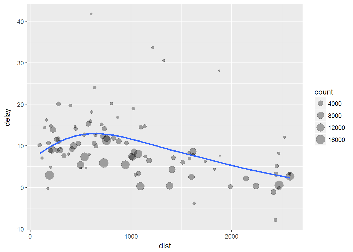
管道式写法:
delays <- flights %>%
  group_by(dest) %>%
  summarise(
    count = n(),
    dist = mean(distance, na.rm = TRUE),
    delay = mean(arr_delay, na.rm = TRUE)
  ) %>%
  filter(count > 20, dest != "HNL")
缺失值
集合型函数的缺失值处理:如果输入中有缺失值,那么输出就是缺失值,除非加na.rm=T。
可以预先筛出没有缺失值的数据。
not_cancelled <- flights %>%
  filter(!is.na(dep_delay), !is.na(arr_delay))

not_cancelled %>%
  group_by(year, month, day) %>%
  summarise(mean = mean(dep_delay))
## # A tibble: 365 x 4
## # Groups: year, month [?]
## year month day mean
## <int> <int> <int> <dbl>
## 1 2013 1 1 11.4
## 2 2013 1 2 13.7
## 3 2013 1 3 10.9
## 4 2013 1 4 8.97
## 5 2013 1 5 5.73
## 6 2013 1 6 7.15
## 7 2013 1 7 5.42
## 8 2013 1 8 2.56
## 9 2013 1 9 2.30
## 10 2013 1 10 2.84
## # ... with 355 more rows计数
当做数据聚合时,最好加一个计数列,保证不是基于很小的数据量做出的结论。
比如在分析每个飞机的延误时间时
delays <- not_cancelled %>%
  group_by(tailnum) %>%
  summarise(
    delay = mean(arr_delay)
  )

ggplot(data = delays, mapping = aes(x = delay)) +
  geom_freqpoly(binwidth = 10)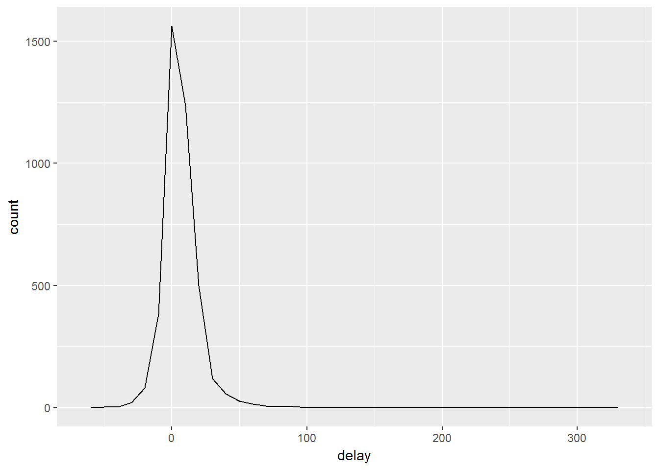
发现有飞机平均延误超过了300分钟。
画出每架飞机航班数和延误的关系
delays <- not_cancelled %>%
  group_by(tailnum) %>%
  summarise(
    delay = mean(arr_delay, na.rm = TRUE),
    n = n()
  )

ggplot(data = delays, mapping = aes(x = n, y = delay)) +
  geom_point(alpha = 1/10)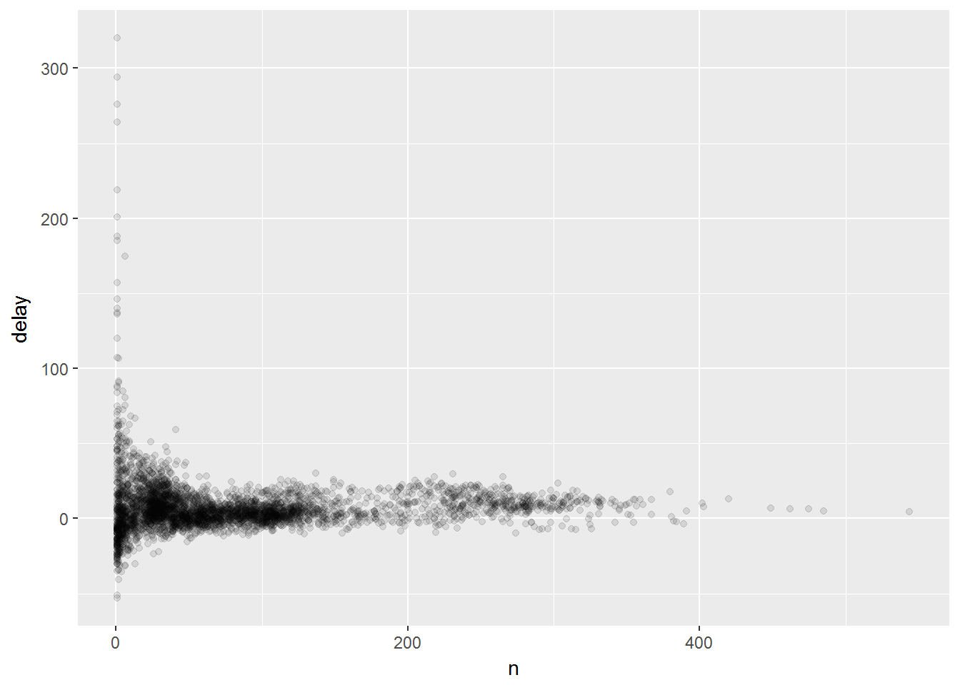
当航班数很小时,数据的方差就很大。随着数据规模增大,方差就会变小。
所以在聚合数据时,通常剔除聚合后样本量很小的数据子集
delays %>%
  filter(n > 25) %>%
  ggplot(mapping = aes(x = n, y = delay)) +
    geom_point(alpha = 1/10)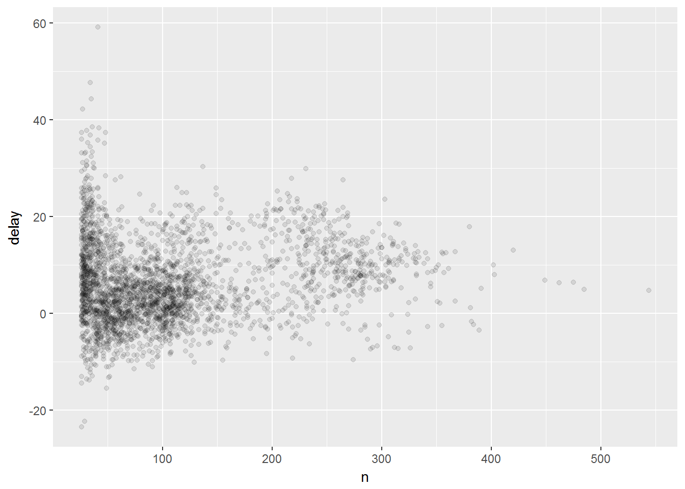
- 计数非缺失值时用sum(!is.na(x))
- 计数unique值时用n_distinct(x)
not_cancelled %>%
  group_by(dest) %>%
  summarise(carriers = n_distinct(carrier)) %>%
  arrange(desc(carriers))
## # A tibble: 104 x 2
## dest carriers
## <chr> <int>
## 1 ATL 7
## 2 BOS 7
## 3 CLT 7
## 4 ORD 7
## 5 TPA 7
## 6 AUS 6
## 7 DCA 6
## 8 DTW 6
## 9 IAD 6
## 10 MSP 6
## # ... with 94 more rowscount()函数单纯用来计数
not_cancelled %>%
  count(dest)
## # A tibble: 104 x 2
## dest n
## <chr> <int>
## 1 ABQ 254
## 2 ACK 264
## 3 ALB 418
## 4 ANC 8
## 5 ATL 16837
## 6 AUS 2411
## 7 AVL 261
## 8 BDL 412
## 9 BGR 358
## 10 BHM 269
## # ... with 94 more rows相当于table
table(not_cancelled$dest)##
## ABQ ACK ALB ANC ATL AUS AVL BDL BGR BHM BNA BOS
## 254 264 418 8 16837 2411 261 412 358 269 6084 15022
## BQN BTV BUF BUR BWI BZN CAE CAK CHO CHS CLE CLT
## 888 2510 4570 370 1687 35 106 842 46 2759 4394 13674
## CMH CRW CVG DAY DCA DEN DFW DSM DTW EGE EYW FLL
## 3326 134 3725 1399 9111 7169 8388 523 9031 207 17 11897
## GRR GSO GSP HDN HNL HOU IAD IAH ILM IND JAC JAX
## 728 1492 790 14 701 2083 5383 7085 107 1981 21 2623
## LAS LAX LEX LGB MCI MCO MDW MEM MHT MIA MKE MSN
## 5952 16026 1 661 1885 13967 4025 1686 932 11593 2709 556
## MSP MSY MTJ MVY MYR OAK OKC OMA ORD ORF PBI PDX
## 6929 3715 14 210 58 309 315 817 16566 1434 6487 1342
## PHL PHX PIT PSE PSP PVD PWM RDU RIC ROC RSW SAN
## 1541 4606 2746 358 18 358 2288 7770 2346 2358 3502 2709
## SAT SAV SBN SDF SEA SFO SJC SJU SLC SMF SNA SRQ
## 659 749 10 1104 3885 13173 328 5773 2451 282 812 1201
## STL STT SYR TPA TUL TVC TYS XNA
## 4142 518 1707 7390 294 95 578 992count可以加权重,就变成了sum
not_cancelled %>%
  count(tailnum, wt= distance)
## # A tibble: 4,037 x 2
## tailnum n
## <chr> <dbl>
## 1 D942DN 3418
## 2 N0EGMQ 239143
## 3 N10156 109664
## 4 N102UW 25722
## 5 N103US 24619
## 6 N104UW 24616
## 7 N10575 139903
## 8 N105UW 23618
## 9 N107US 21677
## 10 N108UW 32070
## # ... with 4,027 more rows这么写更加直白一些
not_cancelled %>%
  group_by(tailnum) %>%
  summarise(sum(distance))
## # A tibble: 4,037 x 2
## tailnum `sum(distance)`
## <chr> <dbl>
## 1 D942DN 3418
## 2 N0EGMQ 239143
## 3 N10156 109664
## 4 N102UW 25722
## 5 N103US 24619
## 6 N104UW 24616
## 7 N10575 139903
## 8 N105UW 23618
## 9 N107US 21677
## 10 N108UW 32070
## # ... with 4,027 more rows对于逻辑值sum()就是统计TRUE的数量,mean()就是统计TRUE的百分比
not_cancelled %>%
  group_by(year, month, day) %>%
  summarise(n_early = sum(dep_time < 500))
## # A tibble: 365 x 4
## # Groups: year, month [?]
## year month day n_early
## <int> <int> <int> <int>
## 1 2013 1 1 0
## 2 2013 1 2 3
## 3 2013 1 3 4
## 4 2013 1 4 3
## 5 2013 1 5 3
## 6 2013 1 6 2
## 7 2013 1 7 2
## 8 2013 1 8 1
## 9 2013 1 9 3
## 10 2013 1 10 3
## # ... with 355 more rowsnot_cancelled %>%
group_by(year, month, day) %>%
summarise(hour_perc = mean(arr_delay > 60))## # A tibble: 365 x 4
## # Groups: year, month [?]
## year month day hour_perc
## <int> <int> <int> <dbl>
## 1 2013 1 1 0.0722
## 2 2013 1 2 0.0851
## 3 2013 1 3 0.0567
## 4 2013 1 4 0.0396
## 5 2013 1 5 0.0349
## 6 2013 1 6 0.0470
## 7 2013 1 7 0.0333
## 8 2013 1 8 0.0213
## 9 2013 1 9 0.0202
## 10 2013 1 10 0.0183
## # ... with 355 more rows上卷
当使用多个分组变量时,可以完成渐进上卷的操作
daily <- group_by(flights, year, month, day)
(per_day   <- summarise(daily, flights = n()))
## # A tibble: 365 x 4
## # Groups: year, month [?]
## year month day flights
## <int> <int> <int> <int>
## 1 2013 1 1 842
## 2 2013 1 2 943
## 3 2013 1 3 914
## 4 2013 1 4 915
## 5 2013 1 5 720
## 6 2013 1 6 832
## 7 2013 1 7 933
## 8 2013 1 8 899
## 9 2013 1 9 902
## 10 2013 1 10 932
## # ... with 355 more rows(per_month <- summarise(per_day, flights = sum(flights)))## # A tibble: 12 x 3
## # Groups: year [?]
## year month flights
## <int> <int> <int>
## 1 2013 1 27004
## 2 2013 2 24951
## 3 2013 3 28834
## 4 2013 4 28330
## 5 2013 5 28796
## 6 2013 6 28243
## 7 2013 7 29425
## 8 2013 8 29327
## 9 2013 9 27574
## 10 2013 10 28889
## 11 2013 11 27268
## 12 2013 12 28135(per_year <- summarise(per_month, flights = sum(flights)))## # A tibble: 1 x 2
## year flights
## <int> <int>
## 1 2013 336776移除分组
daily %>%
  ungroup() %>%
  summarise(flights = n())
## # A tibble: 1 x 1
## flights
## <int>
## 1 336776分组mutate()和filter()
寻找每组中最糟糕的值
flights_sml <- select(flights,
  year:day,
  ends_with("delay"),
  distance,
  air_time
)
flights_sml %>%
  group_by(year, month, day) %>%
  filter(rank(desc(arr_delay)) < 10)
## # A tibble: 3,306 x 7
## # Groups: year, month, day [365]
## year month day dep_delay arr_delay distance air_time
## <int> <int> <int> <dbl> <dbl> <dbl> <dbl>
## 1 2013 1 1 853 851 184 41
## 2 2013 1 1 290 338 1134 213
## 3 2013 1 1 260 263 266 46
## 4 2013 1 1 157 174 213 60
## 5 2013 1 1 216 222 708 121
## 6 2013 1 1 255 250 589 115
## 7 2013 1 1 285 246 1085 146
## 8 2013 1 1 192 191 199 44
## 9 2013 1 1 379 456 1092 222
## 10 2013 1 2 224 207 550 94
## # ... with 3,296 more rows寻找大于某个阈值的分组
popular_dests <- flights %>%
  group_by(dest) %>%
  filter(n() > 365)
popular_dests
## # A tibble: 332,577 x 19
## # Groups: dest [77]
## year month day dep_time sched_dep_time dep_delay arr_time
## <int> <int> <int> <int> <int> <dbl> <int>
## 1 2013 1 1 517 515 2 830
## 2 2013 1 1 533 529 4 850
## 3 2013 1 1 542 540 2 923
## 4 2013 1 1 544 545 -1 1004
## 5 2013 1 1 554 600 -6 812
## 6 2013 1 1 554 558 -4 740
## 7 2013 1 1 555 600 -5 913
## 8 2013 1 1 557 600 -3 709
## 9 2013 1 1 557 600 -3 838
## 10 2013 1 1 558 600 -2 753
## # ... with 332,567 more rows, and 12 more variables: sched_arr_time <int>,
## # arr_delay <dbl>, carrier <chr>, flight <int>, tailnum <chr>,
## # origin <chr>, dest <chr>, air_time <dbl>, distance <dbl>, hour <dbl>,
## # minute <dbl>, time_hour <dttm>分组标准化计算
popular_dests %>%
  filter(arr_delay > 0) %>%
  mutate(prop_delay = arr_delay / sum(arr_delay)) %>%
  select(year:day, dest, arr_delay, prop_delay)
## # A tibble: 131,106 x 6
## # Groups: dest [77]
## year month day dest arr_delay prop_delay
## <int> <int> <int> <chr> <dbl> <dbl>
## 1 2013 1 1 IAH 11 0.000111
## 2 2013 1 1 IAH 20 0.000201
## 3 2013 1 1 MIA 33 0.000235
## 4 2013 1 1 ORD 12 0.0000424
## 5 2013 1 1 FLL 19 0.0000938
## 6 2013 1 1 ORD 8 0.0000283
## 7 2013 1 1 LAX 7 0.0000344
## 8 2013 1 1 DFW 31 0.000282
## 9 2013 1 1 ATL 12 0.0000400
## 10 2013 1 1 DTW 16 0.000116
## # ... with 131,096 more rows在script里,用ctrl+enter执行某一句。