library(tidyverse)这本书是哈德利的入门之作。虽然对于我来说有点过于简单,不过这本书是以系统的观点阐述数据分析中的各个问题,并且都是用tidyverse工具箱中的包解决的。利用闲暇时间读一遍能够系统学习一边tidyverse,也不算浪费时间。不过这本书过的速度可以稍微快一点,毕竟很多都是太基础的内容。
3. 数据可视化
ggplot2的基础语法
ggplot(data = <DATA>) +
  <GEOM_FUNCTION>(
     mapping = aes(<MAPPINGS>),
     stat = <STAT>,
     position = <POSITION>
  ) +
  <COORDINATE_FUNCTION> +
  <FACET_FUNCTION>
样例数据:mpg
str(mpg)## Classes 'tbl_df', 'tbl' and 'data.frame': 234 obs. of 11 variables:
## $ manufacturer: chr "audi" "audi" "audi" "audi" ...
## $ model : chr "a4" "a4" "a4" "a4" ...
## $ displ : num 1.8 1.8 2 2 2.8 2.8 3.1 1.8 1.8 2 ...
## $ year : int 1999 1999 2008 2008 1999 1999 2008 1999 1999 2008 ...
## $ cyl : int 4 4 4 4 6 6 6 4 4 4 ...
## $ trans : chr "auto(l5)" "manual(m5)" "manual(m6)" "auto(av)" ...
## $ drv : chr "f" "f" "f" "f" ...
## $ cty : int 18 21 20 21 16 18 18 18 16 20 ...
## $ hwy : int 29 29 31 30 26 26 27 26 25 28 ...
## $ fl : chr "p" "p" "p" "p" ...
## $ class : chr "compact" "compact" "compact" "compact" ...summary(mpg)## manufacturer model displ year
## Length:234 Length:234 Min. :1.600 Min. :1999
## Class :character Class :character 1st Qu.:2.400 1st Qu.:1999
## Mode :character Mode :character Median :3.300 Median :2004
## Mean :3.472 Mean :2004
## 3rd Qu.:4.600 3rd Qu.:2008
## Max. :7.000 Max. :2008
## cyl trans drv cty
## Min. :4.000 Length:234 Length:234 Min. : 9.00
## 1st Qu.:4.000 Class :character Class :character 1st Qu.:14.00
## Median :6.000 Mode :character Mode :character Median :17.00
## Mean :5.889 Mean :16.86
## 3rd Qu.:8.000 3rd Qu.:19.00
## Max. :8.000 Max. :35.00
## hwy fl class
## Min. :12.00 Length:234 Length:234
## 1st Qu.:18.00 Class :character Class :character
## Median :24.00 Mode :character Mode :character
## Mean :23.44
## 3rd Qu.:27.00
## Max. :44.00“The greatest value of a picture is when it forces us to notice what we never expected to see.” — John Tukey
可映射的图形属性
- color
- size
- shape
- alpha
+加号必须放在一句的末尾而不是下一句的开始。
分面
对分类数据很有用
单一变量的分面:facet_wrap()
ggplot(data = mpg) +
  geom_point(mapping = aes(x = displ, y = hwy)) +
  facet_wrap(~ class, nrow = 2)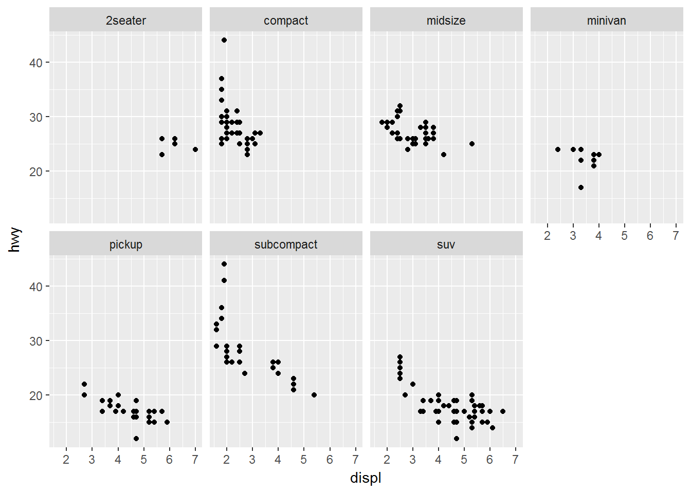
多变量分面:facet_grid()
ggplot(data = mpg) +
  geom_point(mapping = aes(x = displ, y = hwy)) +
  facet_grid(drv ~ cyl)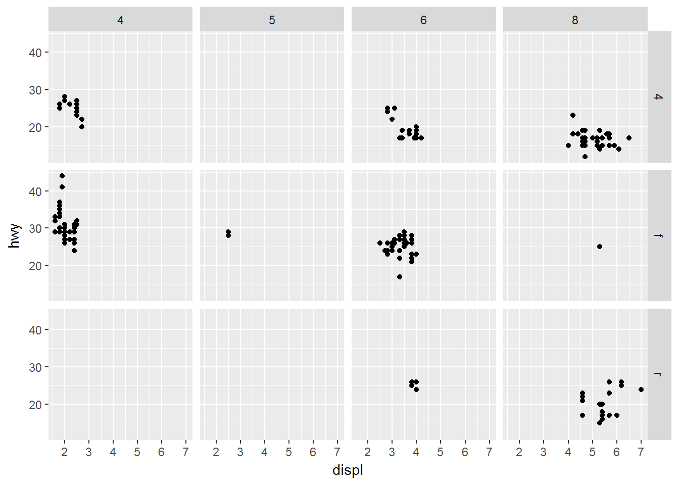
ggplot(data = mpg) +
  geom_point(mapping = aes(x = displ, y = hwy)) +
  facet_grid(. ~ cyl)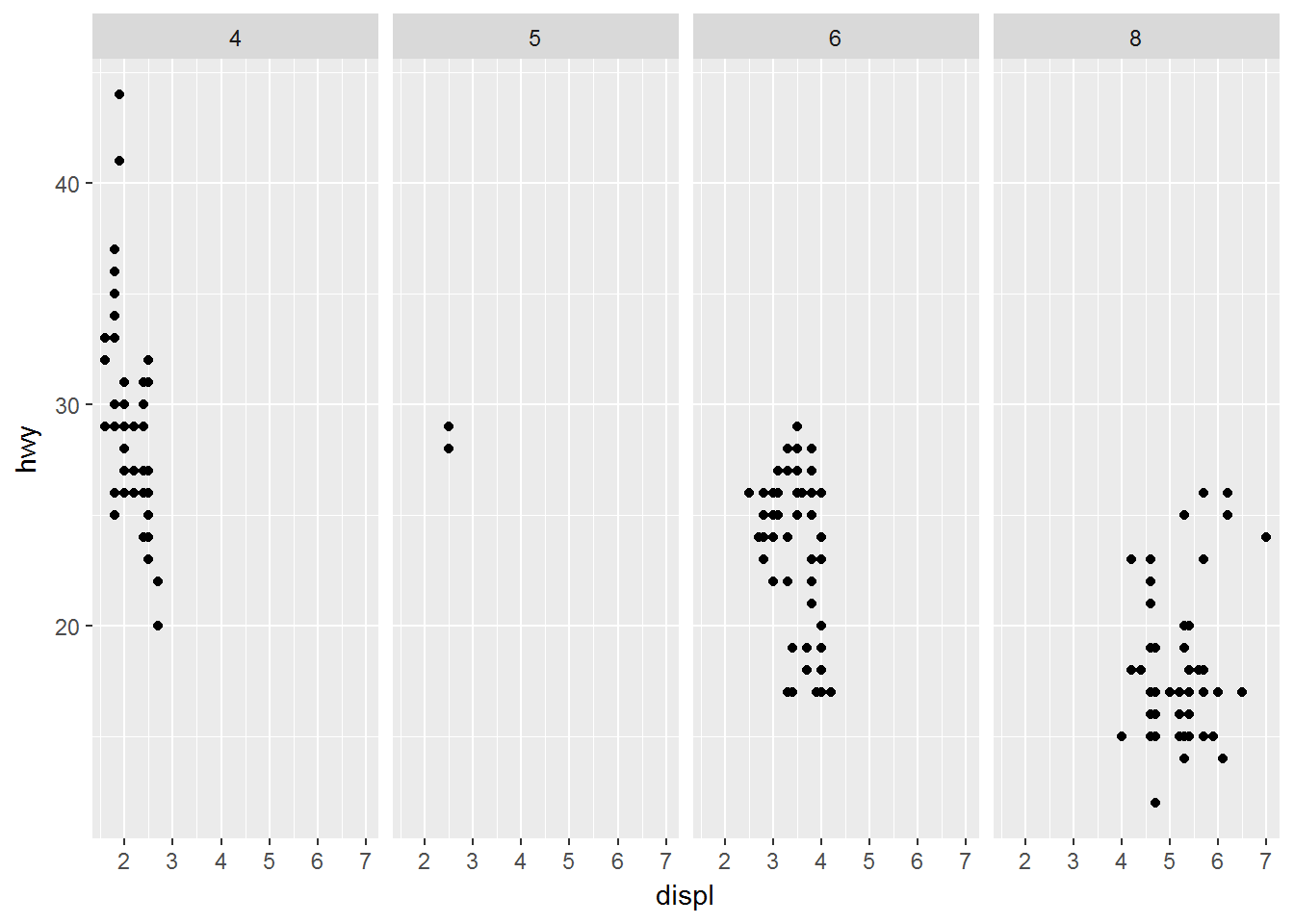
ggplot(data = mpg) +
  geom_point(mapping = aes(x = displ, y = hwy)) +
  facet_grid(drv ~ .)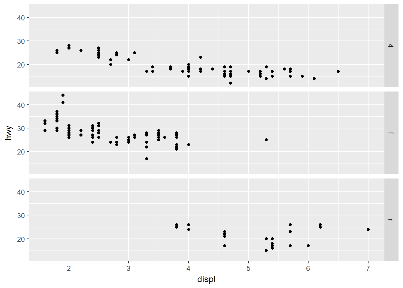
图形类型
ggplot(data = mpg) +
  geom_smooth(mapping = aes(x = displ, y = hwy, linetype = drv))
## `geom_smooth()` using method = 'loess'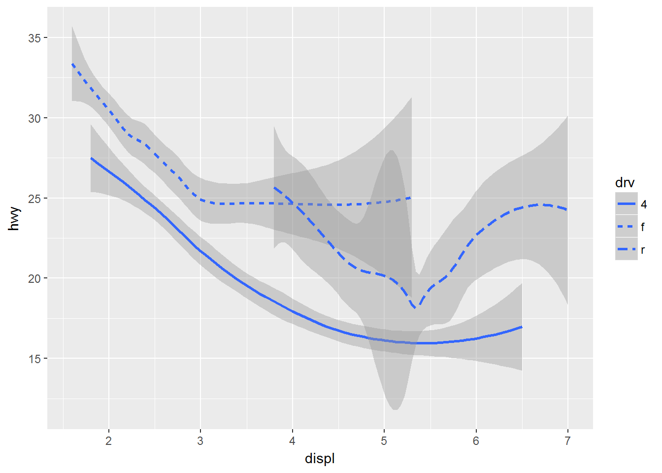
多个图形
ggplot(data = mpg) +
  geom_point(mapping = aes(x = displ, y = hwy)) +
  geom_smooth(mapping = aes(x = displ, y = hwy))
## `geom_smooth()` using method = 'loess'
避免重复的写法:
ggplot(data = mpg, mapping = aes(x = displ, y = hwy)) +
  geom_point() +
  geom_smooth()
## `geom_smooth()` using method = 'loess'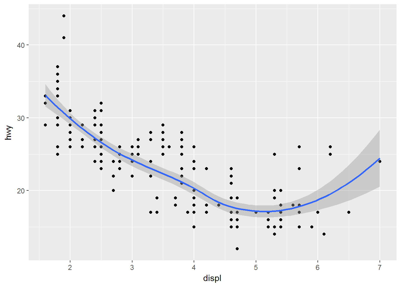
映射的重写
ggplot(data = mpg, mapping = aes(x = displ, y = hwy)) +
  geom_point(mapping = aes(color = class)) +
  geom_smooth()
## `geom_smooth()` using method = 'loess'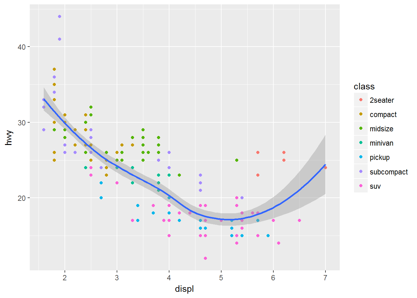
甚至数据也能重写
ggplot(data = mpg, mapping = aes(x = displ, y = hwy)) +
  geom_point(mapping = aes(color = class)) +
  geom_smooth(data = filter(mpg, class == "subcompact"), se = FALSE)
## `geom_smooth()` using method = 'loess'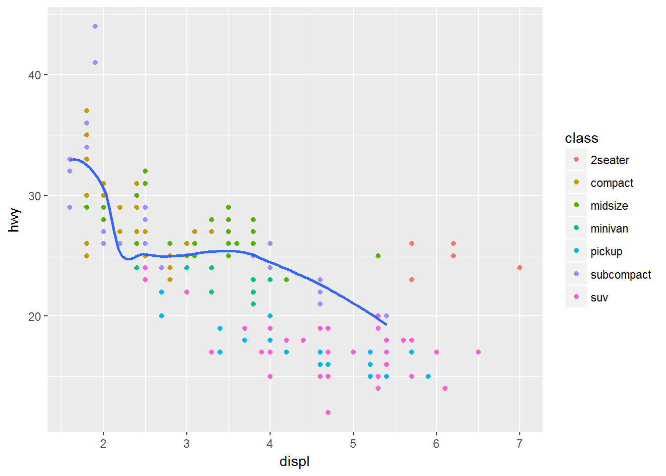
p1 <- ggplot(mpg,aes(x=displ,y=hwy))+
  geom_point()+
  geom_smooth()
p2 <- ggplot(mpg,aes(x=displ,y=hwy))+
  geom_point()+
  geom_smooth(aes(group=drv))
usefulr::multiplot(p1,p2,cols = 2)
## `geom_smooth()` using method = 'loess'
## `geom_smooth()` using method = 'loess'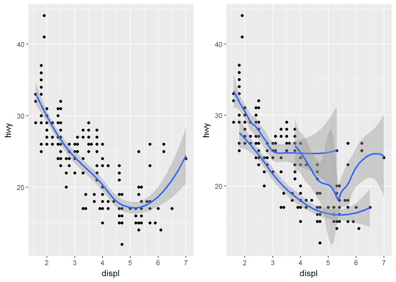
数学变换
ggplot(data = diamonds) +
  geom_bar(mapping = aes(x = cut))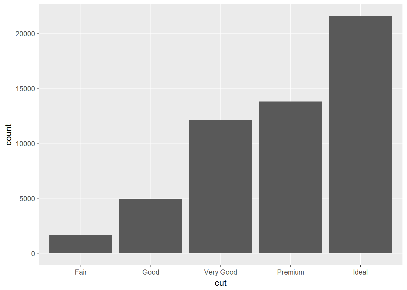
- bar charts, histograms, and frequency polygons bin your data and then plot bin counts, the number of points that fall in each bin.
- smoothers fit a model to your data and then plot predictions from the model.
- boxplots compute a robust summary of the distribution and then display a specially formatted box.
数学变换和图形的关系:
Every geom has a default stat; and every stat has a default geom.
更改图形对应的数学变换:
demo <- tribble(
  ~cut,         ~freq,
  "Fair",       1610,
  "Good",       4906,
  "Very Good",  12082,
  "Premium",    13791,
  "Ideal",      21551
)

ggplot(data = demo) +
  geom_bar(mapping = aes(x = cut, y = freq), stat = "identity")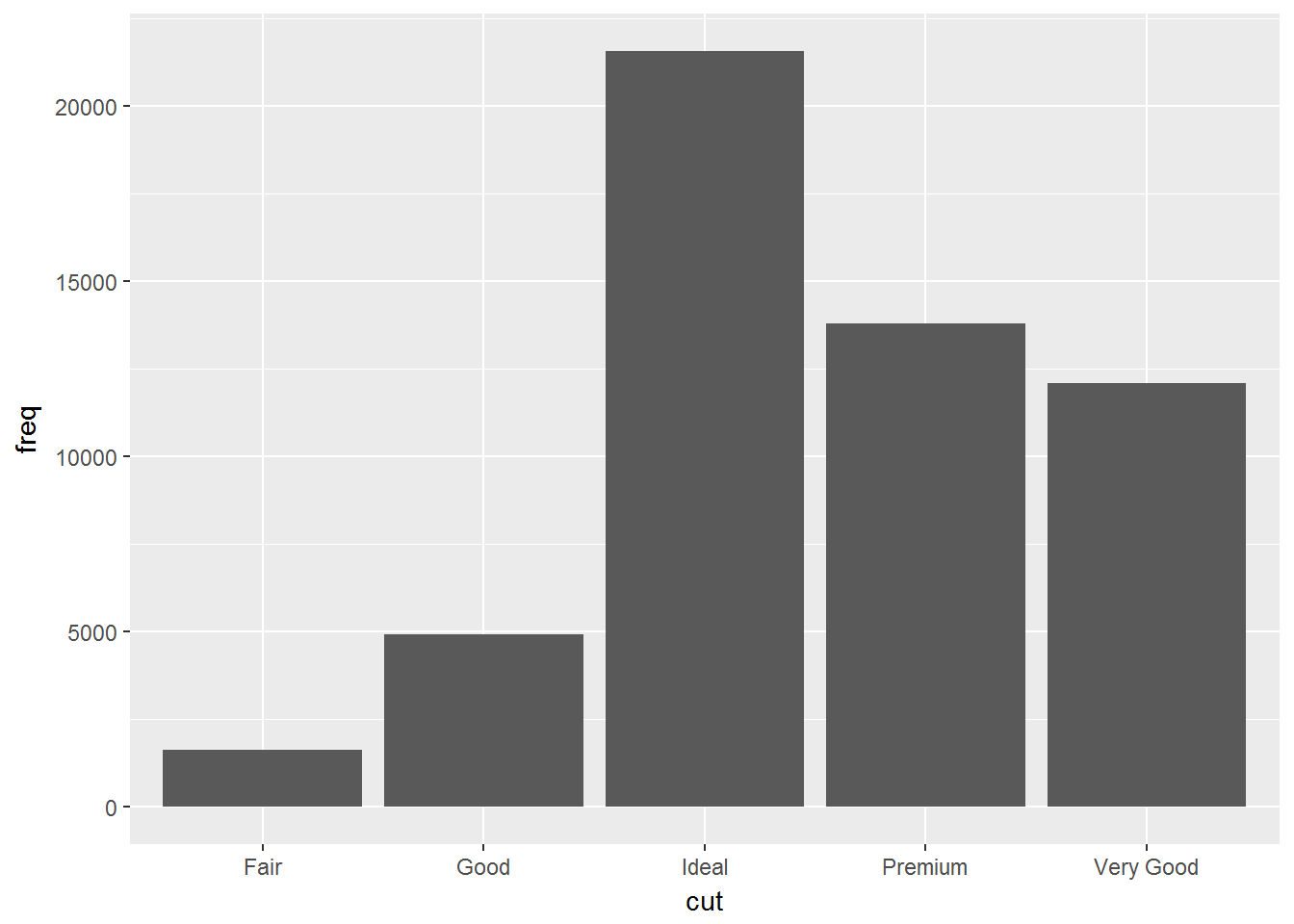
ggplot(data = diamonds) +
  geom_bar(mapping = aes(x = cut, y = ..prop.., group = 1))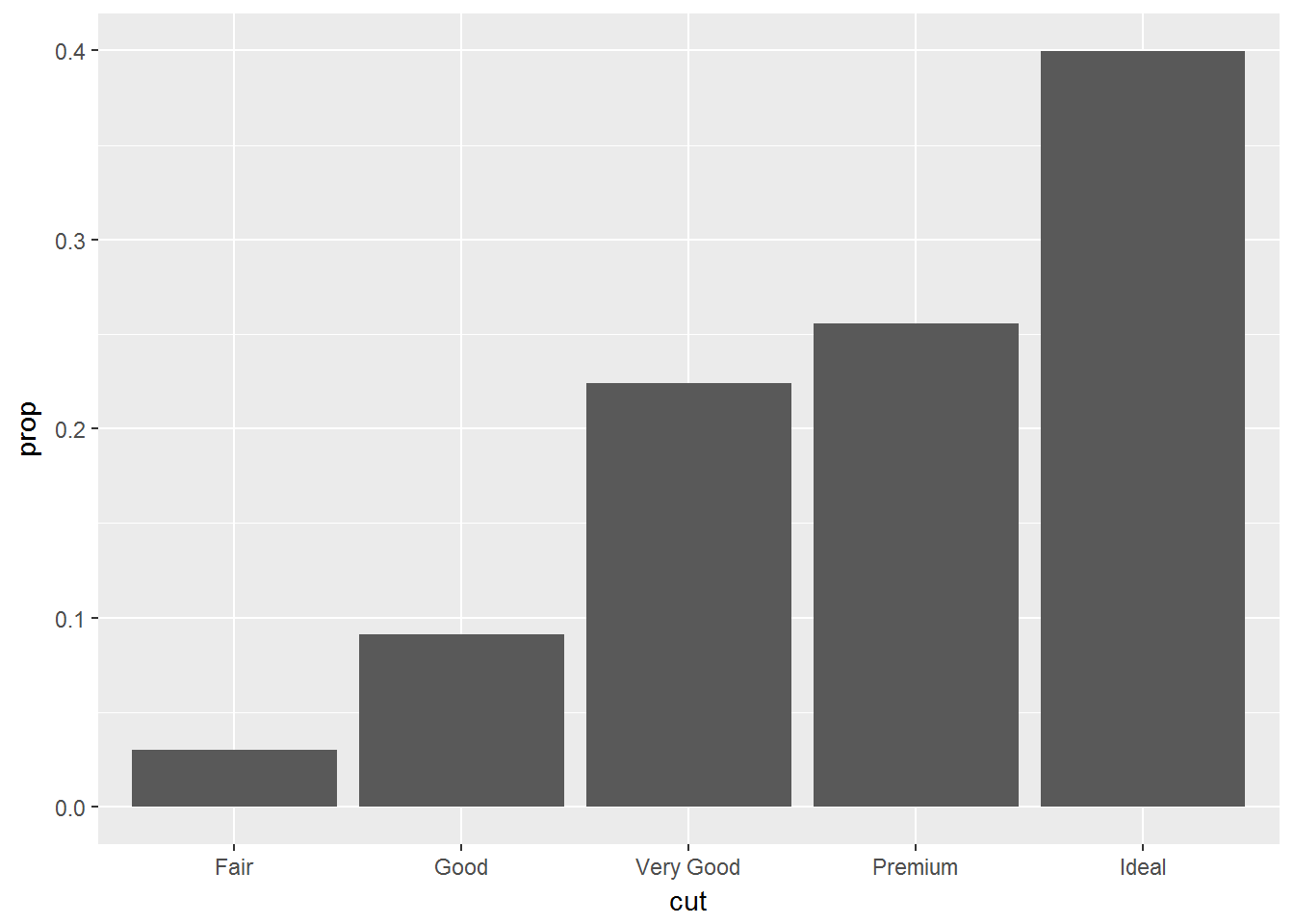
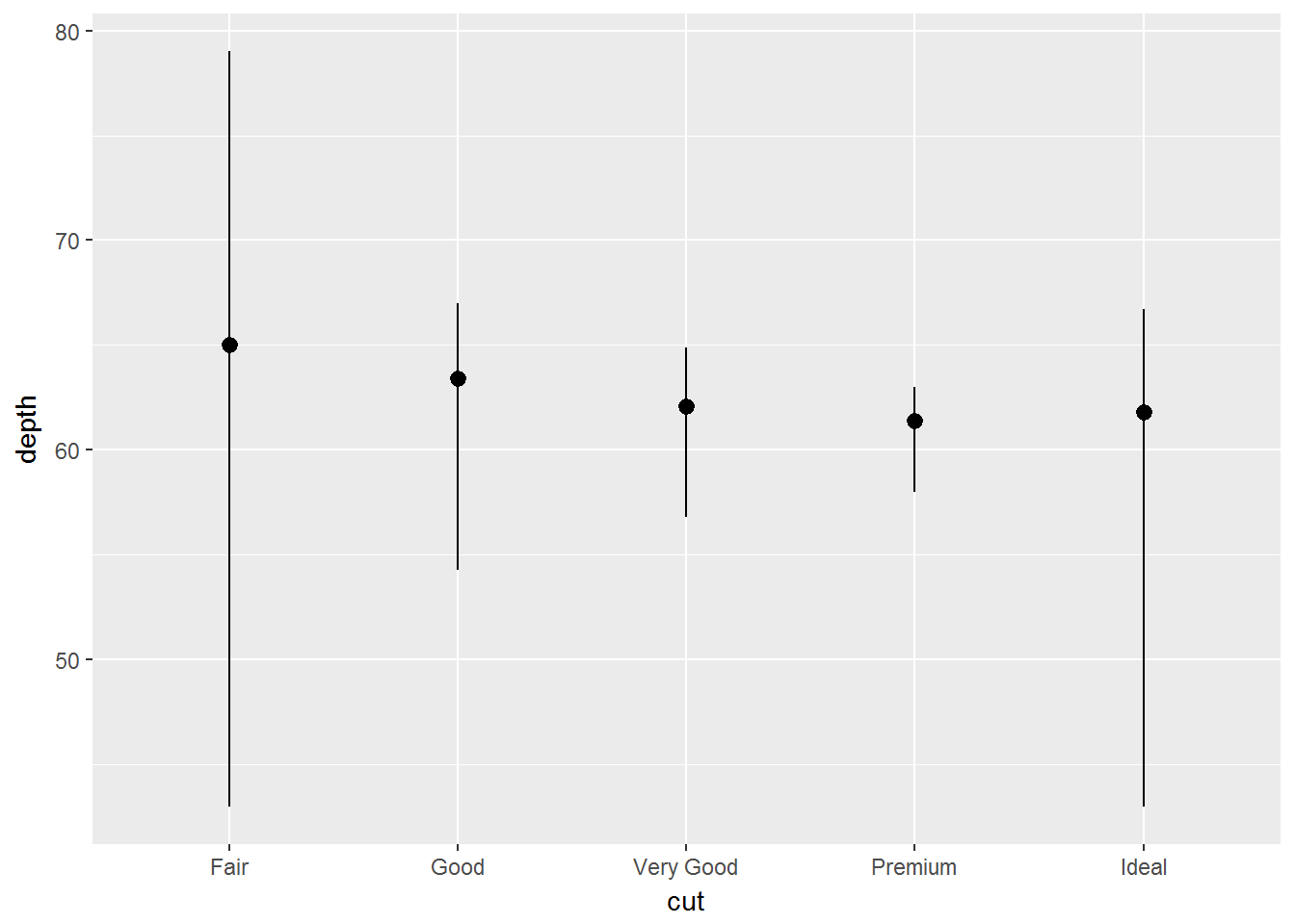
ggplot(data = diamonds) +
  stat_summary(
    mapping = aes(x = cut, y = depth),
    fun.ymin = min,
    fun.ymax = max,
    fun.y = median
  )
位置调整
ggplot(data = diamonds) +
  geom_bar(mapping = aes(x = cut, colour = cut))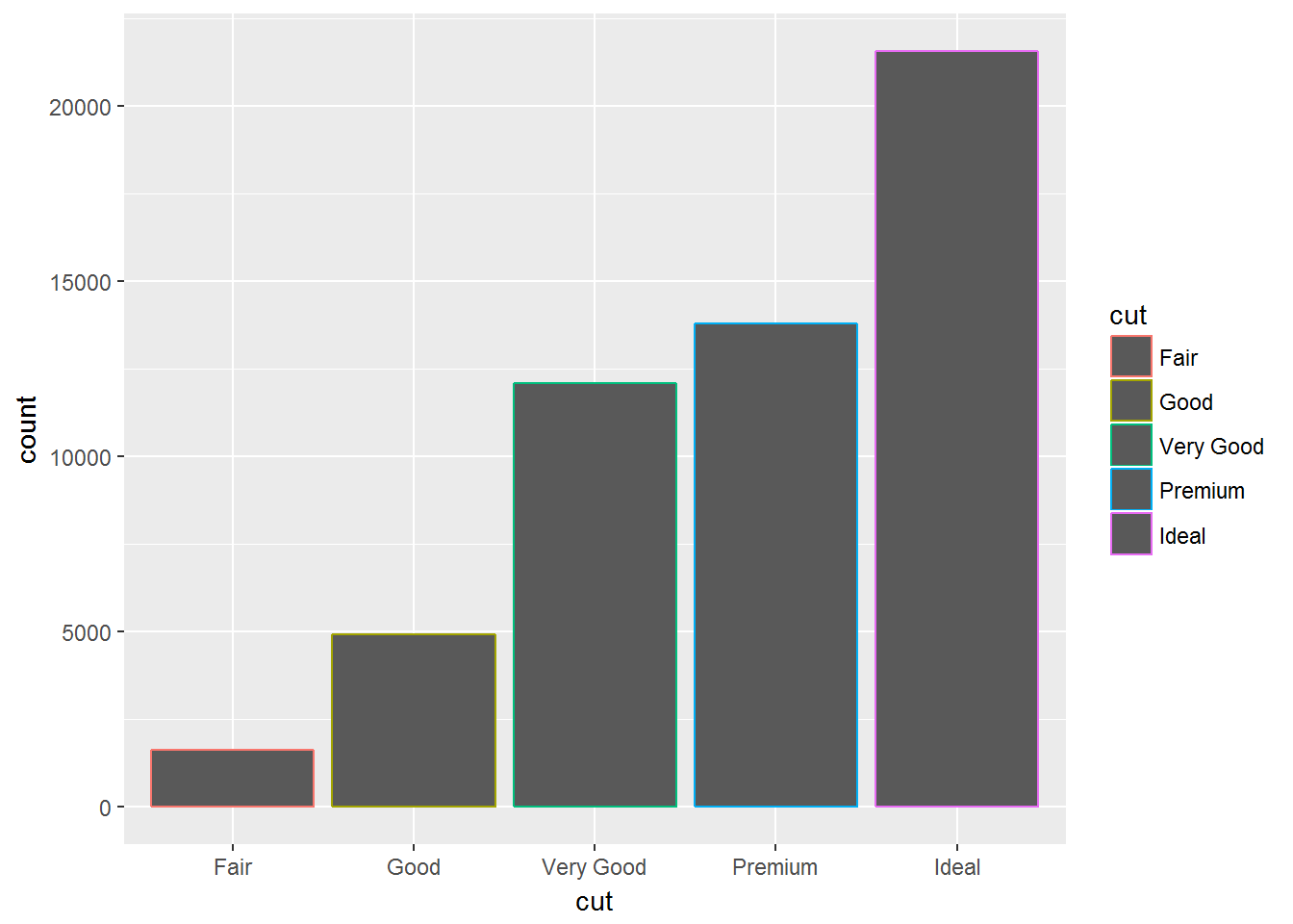
ggplot(data = diamonds) +
  geom_bar(mapping = aes(x = cut, fill = cut))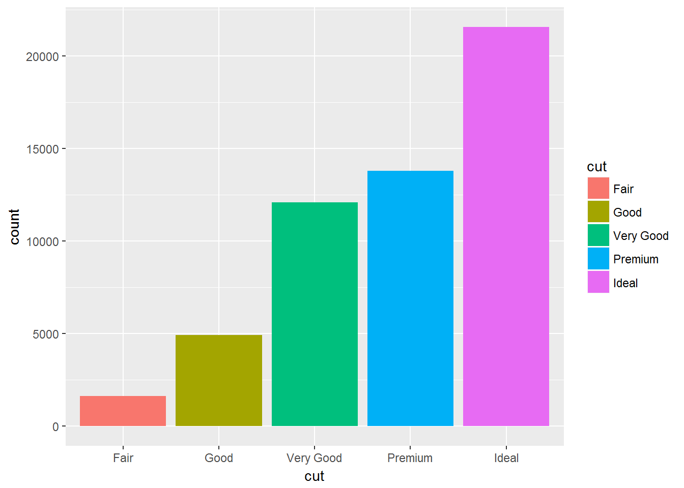
ggplot(data = diamonds) +
  geom_bar(mapping = aes(x = cut, fill = clarity))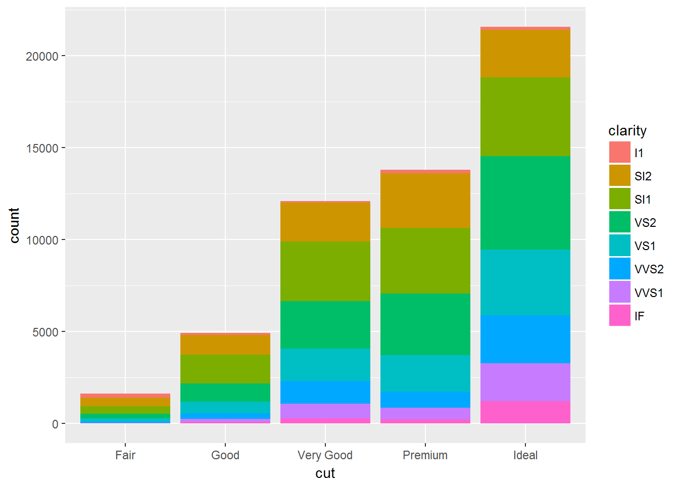
位置调整的四种选择:
- stacked
- identity
- dodge
- fill
- jitter
identity适合展现二维数据
ggplot(data = diamonds, mapping = aes(x = cut, colour = clarity)) +
  geom_bar(fill = NA, position = "identity")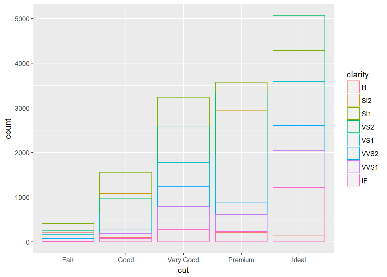
fill适合展现百分比
ggplot(data = diamonds) +
  geom_bar(mapping = aes(x = cut, fill = clarity), position = "fill")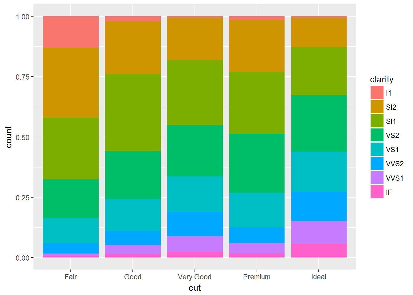
dodge适合展现个体差异
ggplot(data = diamonds) +
  geom_bar(mapping = aes(x = cut, fill = clarity), position = "dodge")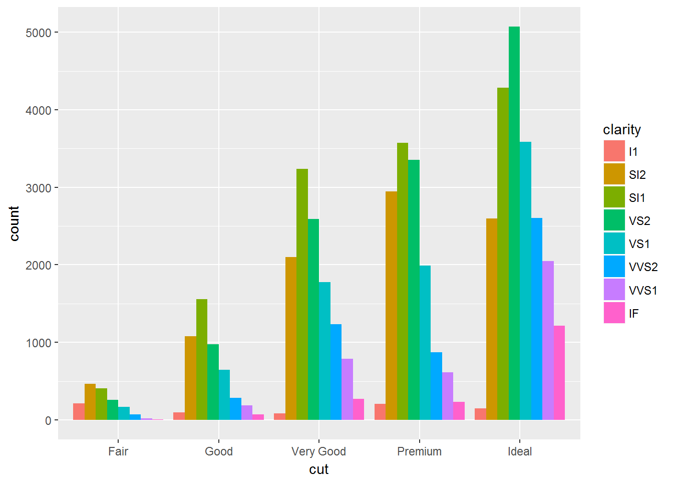
jitter适合展现重叠在一起的大量点,增加扰动
ggplot(data = mpg) +
  geom_point(mapping = aes(x = displ, y = hwy), position = "jitter")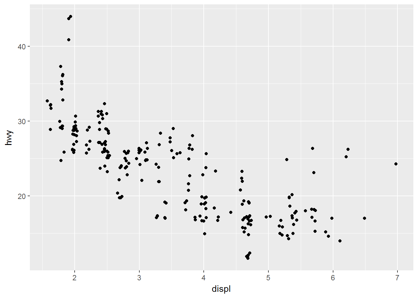
坐标系统
翻转坐标
p1 <- ggplot(data = mpg, mapping = aes(x = class, y = hwy)) +
  geom_boxplot()
p2 <- ggplot(data = mpg, mapping = aes(x = class, y = hwy)) +
  geom_boxplot() +
  coord_flip()
usefulr::multiplot(p1,p2,cols=2)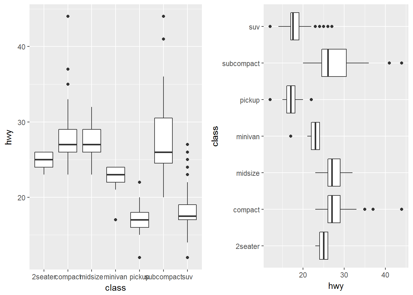
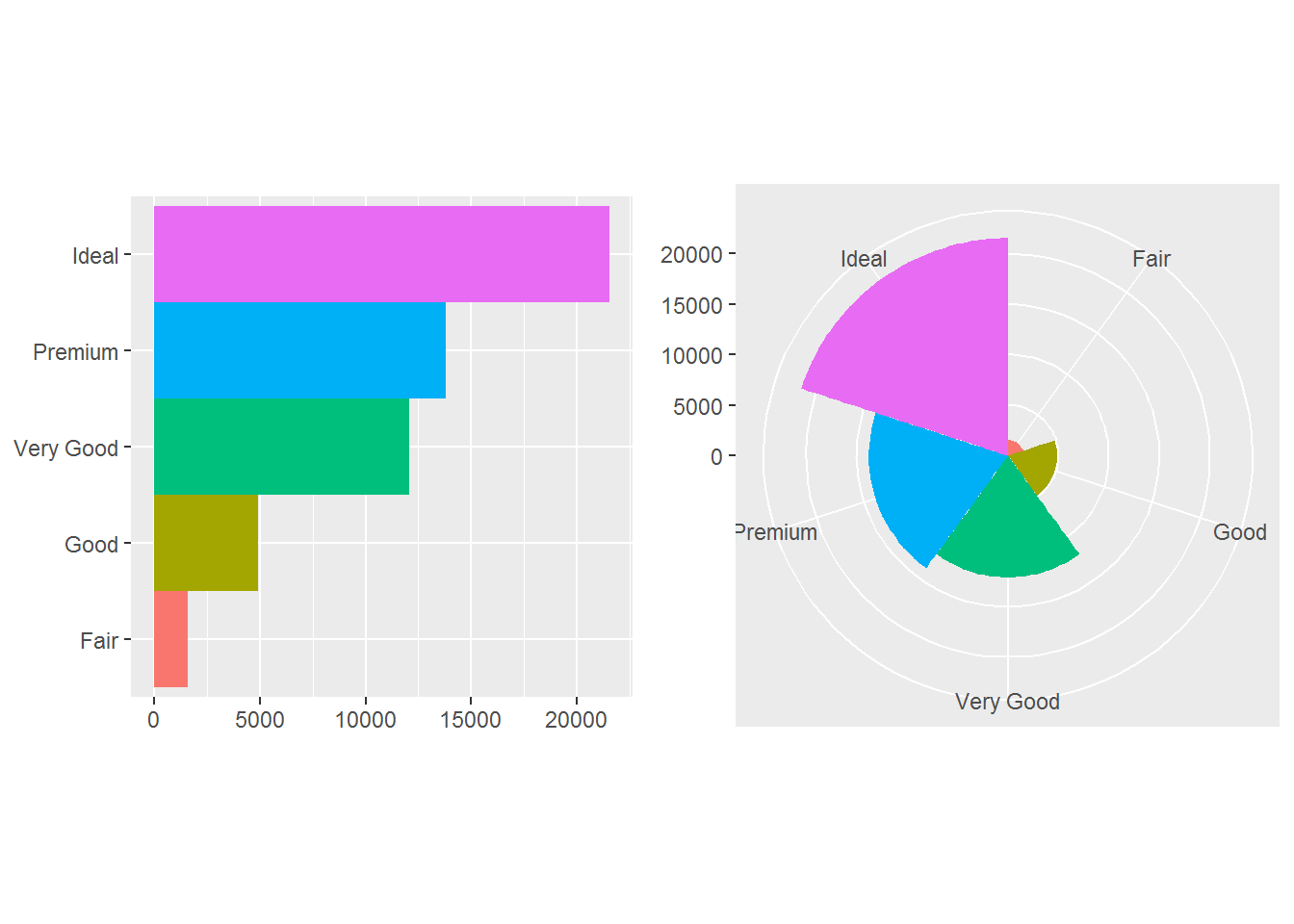
极坐标
bar <- ggplot(data = diamonds) +
  geom_bar(
    mapping = aes(x = cut, fill = cut),
    show.legend = FALSE,
    width = 1
  ) +
  theme(aspect.ratio = 1) +
  labs(x = NULL, y = NULL)
p1 <- bar + coord_flip()
p2 <- bar + coord_polar()
usefulr::multiplot(p1,p2,cols=2)