library(leaflet)
library(leafletCN)
1. 简介
1.1 leaflet的功能
- 交互地图浏览(缩放、平移)
- 使用多种底图进行任意组合
- 加载地图瓦片(WMTS)
- 点要素定位标记
- 多边形要素标记
- 线要素标记
- 弹出窗口
- 解析加载GeoJson
- 从R或者RSutido创建地图窗口
- 可以把地图嵌入 knitr/R包所生成的Markdown文档中,或者是Shiny制作的APP中。
- 可以直接获取通过SP包生成就(加载)的空间对象以及包含经纬度的数据框进行展示。
- 可以设定地图范围以及封装自定义的鼠标事件。
1.2 leaflet的使用步骤
- 加载leaflet包
- 通过leaflet包创建地图控件。
- 通过图层操作的方法(如addTiles、 addMarkers、 addPolygons)来处理图层数据,并且修改地图插件的各种参数,来把图层显示在地图控件上。
- 可以重复第三步,可以增加更多的图层数据。
- 把地图部件显示出来。完成绘图。
m <- leaflet()
at <- addTiles(m)
addMarkers(at,lng = 116.391,lat=39.912,popup = "这里是北京")


管道式写法
leaflet()%>%addTiles()%>%addMarkers(lng=116.391, lat=39.912, popup="这里是北京")2. 地图控件
在leaflet包初始化的时候,一般调用leaflet()这个方法,这个方法就是对地图控件进行初始化,会生成一个地图容器,以后所有的图层操作,都在这个容器内处理。一般来说,这个方法都被作为其他方法的第一个参数来使用。我们可以通过显示参数设定或者通过管道操作符%>%来把这个容器传递给其他的方法。
地图控件的基本方法有下面这三个: - setView() :设定地图的显示级别缩放比例、和地图的中心点。 - fitBounds():设定地图的范围,一般是一个矩形,结构是:[lng1, lat1] – [lng2, lat2]。 - clearBounds():清除地图的范围设定。
m<- leaflet()
m<- setView(m,lng=116.38,lat=39.9,zoom=9)
addTiles(m)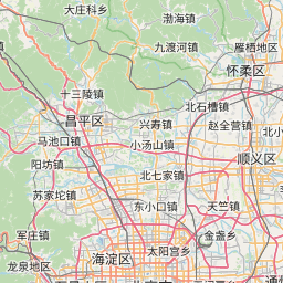


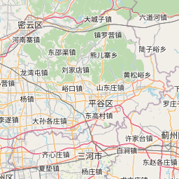

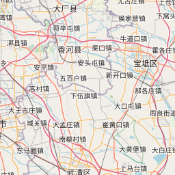
leaflet()%>%setView(lng=116.38,lat=39.9,zoom=9)%>%addTiles()leaflet()%>%setView(lng=116.38,lat=39.9,zoom=3)%>%addTiles()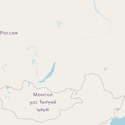

2.1 初始化
leaflet(options = leafletOptions(minZoom = 0, maxZoom = 18))2.2 地图方法
- setView() 设置地图中点和缩放等级;
- fitBounds() 设置显示区域
- clearBounds()
2.3 数据对象
R语言中的:
- 由经纬度信息组成矩阵;
- 带有经纬度字段的数据框。
sp包中的:
- SpatialPoints[DataFrame]
- Line/Lines
- SpatialLines[DataFrame]
- Polygon/Polygons
- SpatialPolygons[DataFrame]
map包中的:
map()所返回的数据框
The data argument is used to derive spatial data for functions that need it; for example, if data is a SpatialPolygonsDataFrame object, then calling addPolygons on that map widget will know to add the polygons from that SpatialPolygonsDataFrame.
It is straightforward to derive these variables from sp objects since they always represent spatial data in the same way. On the other hand, for a normal matrix or data frame, any numeric column could potentially contain spatial data. So we resort to guessing based on column names:
- the latitude variable is guessed by looking for columns named lat or latitude (case-insensitive)
- the longitude variable is guessed by looking for lng, long, or longitude
For example, we do not specify the values for the arguments lat and lng in addCircles() below, but the columns Lat and Long in the data frame df will be automatically used:
# add some circles to a map
df = data.frame(Lat = 1:10, Long = rnorm(10))
leaflet(df) %>% addCircles()You can also explicitly specify the Lat and Long columns (see below for more info on the ~ syntax):
leaflet(df) %>% addCircles(lng = ~Long, lat = ~Lat)A map layer may use a different data object to override the data provided in leaflet(). We can rewrite the above example as:
leaflet() %>% addCircles(data = df)leaflet() %>% addCircles(data = df, lat = ~ Lat, lng = ~ Long)还有就是maps包里面的各种空间图形信息
library(maps)
mapStates = map("state", fill = TRUE, plot = FALSE)
leaflet(data = mapStates) %>% addTiles() %>%
  addPolygons(fillColor = topo.colors(10, alpha = NULL), stroke = FALSE)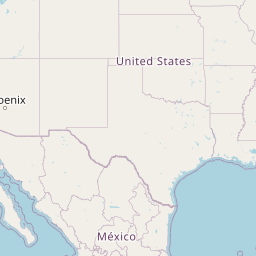


2.4 公式界面
m = leaflet() %>% addTiles()
df = data.frame(
  lat = rnorm(100)*10,
  lng = rnorm(100)*10,
  size = runif(100, 5, 20),
  color = sample(colors(), 100)
)
m = leaflet(df) %>% addTiles()
m %>% addCircleMarkers(radius = ~size, color = ~color, fill = FALSE)
## Assuming "lng" and "lat" are longitude and latitude, respectively


m %>% addCircleMarkers(radius = runif(100, 4, 10), color = c('red'))## Assuming "lng" and "lat" are longitude and latitude, respectively3. 底图
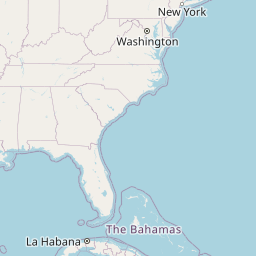
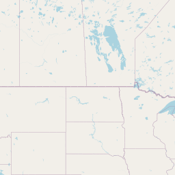
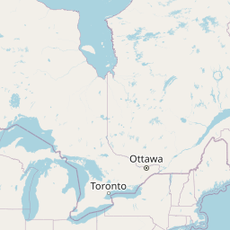
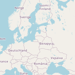
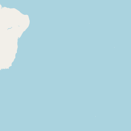
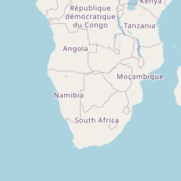
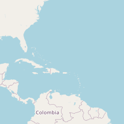
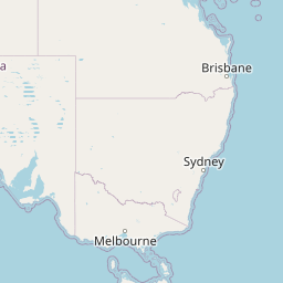
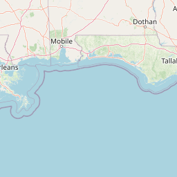
3.1 默认:OpenStreetMap
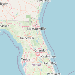
m <- leaflet() %>% setView(lng = -71.0589, lat = 42.3601, zoom = 12)
m %>% addTiles()


3.2 第三方底图
addProviderTiles()
As a convenience, leaflet also provides a named list of all the third-party tile providers that are supported by the plugin. This enables you to use auto-completion feature of your favorite R IDE (like RStudio) and not have to remember or look up supported tile providers; just type providers$ and choose from one of the options. You can also use names(providers) to view all of the options.
providers$OpenStreetMap.CH## [1] "OpenStreetMap.CH"可用底图:
路网
- addTiles()
- amap() 高德
- HikeBike.HikeBike
- Wikimedia
卫星
- Esri.WorldImagery
水彩
- Stamen.Watercolor
4. 标记
Use markers to call out points on the map. Marker locations are expressed in latitude/longitude coordinates, and can either appear as icons or as circles.
4.1 数据源
- SpatialPoints or SpatialPointsDataFrame objects (from the sp package)
- POINT, sfc_POINT, and sf objects (from the sf package); only X and Y dimensions will be considered.
- Two-column numeric matrices (first column is longitude, second is latitude).
- Data frame with latitude and logitude columns. You can explicitly tell the marker function which columns contain the coordinate data (e.g. addMarkers(lng = ~Longitude, lat = ~Latitude)), or let the function look for columns named lat/latitude and lon/lng/long/longitude (case insensitive).
- Simply provide numeric vectors as lng and lat arguments.
4.2 标记
Icon markers are added using the addMarkers or the addAwesomeMarkers functions. Their default appearance is a dropped pin. As with most layer functions, the popup argument can be used to add a message to be displayed on click, and the label option can be used to display a text label either on hover or statically.
addMarkers
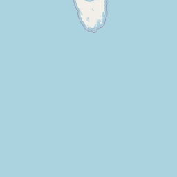
data(quakes)

# Show first 20 rows from the `quakes` dataset
leaflet(data = quakes[1:20,]) %>% addTiles() %>%
  addMarkers(~long, ~lat, popup = ~as.character(mag), label = ~as.character(mag))


addAwesomeMarkers定制化
# first 20 quakes
df.20 <- quakes[1:20,]

getColor <- function(quakes) {
  sapply(quakes$mag, function(mag) {
  if(mag <= 4) {
    "green"
  } else if(mag <= 5) {
    "orange"
  } else {
    "red"
  } })
}

icons <- awesomeIcons(
  icon = 'ios-close',
  iconColor = 'black',
  library = 'ion',
  markerColor = getColor(df.20)
)

leaflet(df.20) %>% addTiles() %>%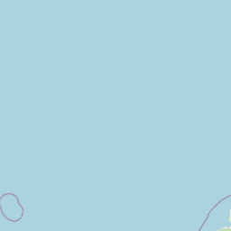
addAwesomeMarkers(~long, ~lat, icon=icons, label=~as.character(mag))聚类
leaflet(quakes) %>% addTiles() %>% addMarkers(
  clusterOptions = markerClusterOptions()
)
## Assuming "long" and "lat" are longitude and latitude, respectively


圆形标记
leaflet(df) %>% addTiles() %>% addCircleMarkers()## Assuming "lng" and "lat" are longitude and latitude, respectively定制化圆形标记
# Create a palette that maps factor levels to colors

# Some fake data
df <- sp::SpatialPointsDataFrame(
  cbind(
    (runif(20) - .5) * 10 - 90.620130,  # lng
    (runif(20) - .5) * 3.8 + 25.638077  # lat
  ),
  data.frame(type = factor(
    ifelse(runif(20) > 0.75, "pirate", "ship"),
    c("ship", "pirate")
  ))
)

pal <- colorFactor(c("navy", "red"), domain = c("ship", "pirate"))

leaflet(df) %>% addTiles() %>%
  addCircleMarkers(
    radius = ~ifelse(type == "ship", 6, 10),
    color = ~pal(type),
    stroke = F, fillOpacity = 0.5
  )


5. 弹窗和标签
5.1 Popups
Popups are small boxes containing arbitrary HTML, that point to a specific point on the map.
Use the addPopups() function to add standalone popup to the map.
content <- paste(sep = "<br/>",
  "<b><a href='http://www.samurainoodle.com'>Samurai Noodle</a></b>",
  "606 5th Ave. S",
  "Seattle, WA 98138"
)

leaflet() %>% addTiles() %>%
  addPopups(-122.327298, 47.597131, content,
    options = popupOptions(closeButton = T)
  )


library(htmltools)

df <- read.csv(textConnection(
"Name,Lat,Long
Samurai Noodle,47.597131,-122.327298
Kukai Ramen,47.6154,-122.327157
Tsukushinbo,47.59987,-122.326726"
))

leaflet(df) %>% addTiles() %>%
  addMarkers(~Long, ~Lat, popup = ~htmlEscape(Name))


In the preceding example, htmltools::htmlEscape was used to santize any characters in the name that might be interpreted as HTML. While it wasn’t necessary for this example (as the restaurant names contained no HTML markup), doing so is important in any situation where the data may come from a file or database, or from the user.
In addition to markers you can also add popups on shapes like lines, circles and other polygons.
5.2 Labels
A label is a textual or HTML content that can attached to markers and shapes to be always displayed or displayed on mouse over. Unlike popups you don’t need to click a marker/polygon for the label to be shown.
library(htmltools)

df <- read.csv(textConnection(
"Name,Lat,Long
Samurai Noodle,47.597131,-122.327298
Kukai Ramen,47.6154,-122.327157
Tsukushinbo,47.59987,-122.326726"))

leaflet(df) %>% addTiles() %>%
addMarkers(~Long, ~Lat, label = ~htmlEscape(Name))定制化标签
# Change Text Size and text Only and also a custom CSS
leaflet() %>% addTiles() %>% setView(-118.456554, 34.09, 13) %>%
  addMarkers(
    lng = -118.456554, lat = 34.105,
    label = "Default Label",
    labelOptions = labelOptions(noHide = T)) %>%
  addMarkers(
    lng = -118.456554, lat = 34.095,
    label = "Label w/o surrounding box",
    labelOptions = labelOptions(noHide = T, textOnly = TRUE)) %>%
  addMarkers(
    lng = -118.456554, lat = 34.085,
    label = "label w/ textsize 15px",
    labelOptions = labelOptions(noHide = T, textsize = "15px")) %>%
  addMarkers(
    lng = -118.456554, lat = 34.075,
    label = "Label w/ custom CSS style",
    labelOptions = labelOptions(noHide = T, direction = "bottom",
      style = list(
        "color" = "red",
        "font-family" = "serif",
        "font-style" = "italic",
        "box-shadow" = "3px 3px rgba(0,0,0,0.25)",
        "font-size" = "12px",
        "border-color" = "rgba(0,0,0,0.5)"
      )))


6. 线条和图形
6.1 多边形和多段线
数据来源
- SpatialPolygons, SpatialPolygonsDataFrame, Polygons, and Polygon objects (from the sp package)
- SpatialLines, SpatialLinesDataFrame, Lines, and Line objects (from the sp package)
- MULTIPOLYGON, POLYGON, MULTILINESTRING, and LINESTRING objects (from the sf package)
- map objects (from the maps package’s map() function); use map(fill = TRUE) for polygons, FALSE for polylines
- Two-column numeric matrix; the first column is longitude and the second is latitude. Polygons are separated by rows of (NA, NA). It is not possible to represent multi-polygons nor polygons with holes using this method; use SpatialPolygons instead.
library(maps)
states <- map("state")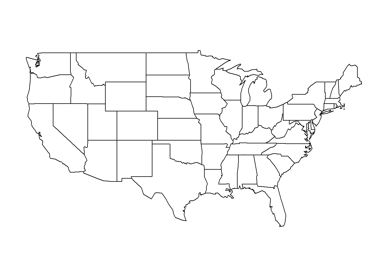
library(rgdal)
# From https://www.census.gov/geo/maps-data/data/cbf/cbf_state.html
states <- readOGR("shp/cb_2013_us_state_20m.shp",
layer = "cb_2013_us_state_20m", GDAL1_integer64_policy = TRUE)
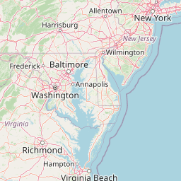
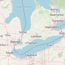
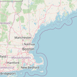
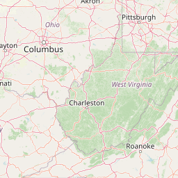
neStates <- subset(states, states$STUSPS %in% c(
"CT","ME","MA","NH","RI","VT","NY","NJ","PA"
))
leaflet(neStates) %>%
addPolygons(color = "#444444", weight = 1, smoothFactor = 0.5,
opacity = 1.0, fillOpacity = 0.5,
fillColor = ~colorQuantile("YlOrRd", ALAND)(ALAND),
highlightOptions = highlightOptions(color = "white", weight = 2,
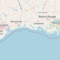
bringToFront = TRUE))6.2 圆形
Circles are added using addCircles(). Circles are similar to circle markers; the only difference is that circles have their radii specified in meters, while circle markers are specified in pixels. As a result, circles are scaled with the map as the user zooms in and out, while circle markers remain a constant size on the screen regardless of zoom level.
cities <- read.csv(textConnection("
City,Lat,Long,Pop
Boston,42.3601,-71.0589,645966
Hartford,41.7627,-72.6743,125017
New York City,40.7127,-74.0059,8406000
Philadelphia,39.9500,-75.1667,1553000
Pittsburgh,40.4397,-79.9764,305841
Providence,41.8236,-71.4222,177994
"))

leaflet(cities) %>% addTiles() %>%addCircles(lng = ~Long, lat = ~Lat, weight = 1,radius = ~sqrt(Pop) * 30, popup = ~City)
6.3 矩形
leaflet() %>% addTiles() %>%
  addRectangles(
    lng1=-118.456554, lat1=34.078039,
    lng2=-118.436383, lat2=34.062717,
    fillColor = "transparent")


7. 颜色
7.1 颜色函数
colorNumeric: 将连续数值线性映射为设定的颜色模式的过程,一般来说,会对设定的颜色模式根据数值的变化进行平滑插值。
colorBin:也是将连续数值线性映射为设定的颜色模式的过程,也会对数据进行平滑内插生成颜色,但是与上一种方法不同的是,这个方法会对设定的颜色模式根据数值的变化进行分级设定。
colorQuantile : 也是线性映射,但是设定的方式是通过百分位数进行分级。
colorFactor: 把分类映射到颜色模式,如果颜色模式设定的数量和分类数量不一样,那么就对颜色模式进行平滑内插。
当然,你也可以使用R语言提供的那些调色板,比如heat.colors、cm.colors、rainbow等等,相关内容请查阅资料。
leaflet里面的颜色设置一共有2个参数,分布是color和fillcolor,从名称就可以看出来,一个是主颜色,一个是填充色,那么对应各种对象来说,color一般就是所谓的边框的颜色了。
Create a vector of n contiguous colors.
- rainbow(n, s = 1, v = 1, start = 0, end = max(1, n - 1)/n, alpha = 1)
- heat.colors(n, alpha = 1)
- terrain.colors(n, alpha = 1)
- topo.colors(n, alpha = 1)
- cm.colors(n, alpha = 1)
参数:
- n:the number of colors (≥ 1) to be in the palette.
- start:the (corrected) hue in [0,1] at which the rainbow begins.
- end:the (corrected) hue in [0,1] at which the rainbow ends.
- alpha:he alpha transparency, a number in [0,1], see argument alpha in hsv.
With rainbow, the parameters start and end can be used to specify particular subranges of hues. The following values can be used when generating such a subrange: red = 0, yellow = 1/6, green = 2/6, cyan = 3/6, blue = 4/6 and magenta = 5/6.
poly <- readShapePoly(paste(path,"CNPG_S.shp",sep =""))

pal <- colorNumeric(c("darkgreen", "yellow", "orangered"),poly@data$Pop_2009)

leaflet(poly) %>% addTiles() %>%
  addPolygons(color=~pal(poly@data$Pop_2009),fillOpacity  = 0.8,weight=1)%>%
  addLegend(pal = pal, values = poly@data$Pop_2009,position="bottomright",title = "2009年人口数量(万人)")


pal <- colorNumeric("Greens",poly@data$Pop_2009)

leaflet(poly) %>% addTiles() %>%
  addPolygons(color=~pal(poly@data$Pop_2009),fillOpacity  = 0.8,weight=1)%>%
  addLegend(pal = pal, values = poly@data$Pop_2009,position="bottomright",title = "2009年人口数量(万人)")


pal <- colorBin(c("darkgreen", "yellow", "orangered"),poly@data$Pop_2009,10)

leaflet(poly) %>% addTiles() %>%
  addPolygons(color=~pal(poly@data$Pop_2009),fillOpacity  = 0.8,weight=1)%>%
  addLegend(pal = pal, values = poly@data$Pop_2009,position="bottomright",title = "2009年人口数量分级")


pal <- colorBin("Greens",poly@data$Pop_2009,10)

leaflet(poly) %>% addTiles() %>%
  addPolygons(color=~pal(poly@data$Pop_2009),fillOpacity  = 0.8,weight=1)%>%
  addLegend(pal = pal, values = poly@data$Pop_2009,position="bottomright",title = "2009年人口数量分级")
8. 图例
addLegend(地图,属性,颜色列表,标记值……)
pal <- colorNumeric("Greens",poly@data$Pop_2009)

leaflet(poly) %>% addTiles() %>%
  addPolygons(color=~pal(poly@data$Pop_2009),fillOpacity  = 0.8,weight=1)%>%
  addLegend(pal = pal, values = poly@data$Pop_2009,title = "2009年人口数量(万人)</br>默认,右上角")%>%

  addLegend(pal = pal, values = poly@data$Pop_2009,bins=5,position="bottomleft",title = "2009年人口数量(万人)</br>图例分级五级,左下角")%>%

  addLegend(pal = pal, values = poly@data$Pop_2009,position="topleft",labFormat = labelFormat(suffix = " 万"),title = "2009年人口数量(万人)</br>加单位,左上角")%>%

  addLegend(pal = pal, values = poly@data$Pop_2009,position="bottomright",opacity = 1,title = "2009年人口数量(万人)</br>色带条不透明,右下角")
9. 图层
9.1 理解分组
A group is a label given to a set of layers. You assign layers to groups by using the group parameter when adding the layers to the map.
leaflet() %>%
  addTiles() %>%
  addMarkers(data = coffee_shops, group = "Food & Drink") %>%
  addMarkers(data = restaurants, group = "Food & Drink") %>%
  addMarkers(data = restrooms, group = "Restrooms")
Many layers can belong to same group. But each layer can only belong to zero or one groups (you can’t assign a layer to two groups).
9.2 交互式图层显示
outline <- quakes[chull(quakes$long, quakes$lat),]

map <- leaflet(quakes) %>%
  # Base groups
  addTiles(group = "OSM (default)") %>%
  addProviderTiles(providers$Stamen.Toner, group = "Toner") %>%
  addProviderTiles(providers$Stamen.TonerLite, group = "Toner Lite") %>%
  # Overlay groups
  addCircles(~long, ~lat, ~10^mag/5, stroke = F, group = "Quakes") %>%
  addPolygons(data = outline, lng = ~long, lat = ~lat,
    fill = F, weight = 2, color = "#FFFFCC", group = "Outline") %>%
  # Layers control
  addLayersControl(
    baseGroups = c("OSM (default)", "Toner", "Toner Lite"),
    overlayGroups = c("Quakes", "Outline"),
    options = layersControlOptions(collapsed = FALSE)
  )
map9.4 与标记聚类一起使用
quakes <- quakes %>%
  dplyr::mutate(mag.level = cut(mag,c(3,4,5,6),
                                labels = c('>3 & <=4', '>4 & <=5', '>5 & <=6')))

quakes.df <- split(quakes, quakes$mag.level)

l <- leaflet() %>% addTiles()

names(quakes.df) %>%
  purrr::walk( function(df) {
    l <<- l %>%
      addMarkers(data=quakes.df[[df]],
                          lng=~long, lat=~lat,
                          label=~as.character(mag),
                          popup=~as.character(mag),
                          group = df,
                          clusterOptions = markerClusterOptions(removeOutsideVisibleBounds = F),
                          labelOptions = labelOptions(noHide = F,
                                                       direction = 'auto'))
  })

l %>%
  addLayersControl(
    overlayGroups = names(quakes.df),
    options = layersControlOptions(collapsed = FALSE)
  )