plyr包是Hadley Wickham在早期创作的一个R包,创作时间大约是2011年左右。这个包的主题思想是“The Split-Apply-Combine Strategy”,我将它翻译为“分而治之的策略”。它是指将一个大问题切分为若干个相似的、并列的小问题。如果能找到小问题的解决办法,那么将其平行的运用在其他小问题上,就解决了整个大问题。Wickham为阐述plyr的使用方法,写了一篇论文,投在《Journal of Statistical Software》开源期刊上,论文名为《The Split-Apply-Combine Strategy for Data Analysis》。本文便是这篇论文的学习笔记。
PS:通过这一篇论文的学习,我认为叫“化整为零的策略”似乎更贴切。
1. 引言
分而治之的策略可以应用在数据挖掘的多个阶段中:
- 在数据预处理阶段,进行分组的排序,标准化,正则化或创建基于组的新变量;
- 在数据探索阶段,计算分组的统计量和其他分析与可视化展示;
- 在建模阶段,建立分组的模型。这些模型可能本身就很有价值,或者一起构建更加复杂的分层模型。
分而治之的策略和谷歌提出的map-reduce的策略很像。Map-reduce是应用在大规模计算集群上的。
这样的分组计算在其他统计软件上也很常见:Excel的透视表,SQL的group by语句等等。plyr就是这样的R包。plyr能够简化循环,并且忽略数据结构上的差异。
plyr的应用作了如下背景假设:
- 数据中的每一小份都只被计算一次,这意味着如果数据是重叠的就没法应用。
- 每一次计算独立于其他计算;计算过程不是迭代的。
注意:
本文所说的数组(Array)包括了一维数组vectors和二维数组matrices。数组可以是原子的(Logical,character,integer,numeric);也可以是列表数组(list-array),实际上它是带维度的列表,可以包含不同种类的数据结构。
2. 动机
本章主要是论述plyr包的函数相比循环和apply家族函数,更加简洁清晰。
3, 使用方法
| Input\ Output | Array | Data frame | List | Discarded |
|---|---|---|---|---|
| Array | aaply | adply | alply | a_ply |
| Data Frame | daply | ddply | dlply | d_ply |
| List | laply | ldply | llply | l_ply |
3.1 输入
输入决定了怎样切分数据。
a*ply()
按维度切分数据,将数据切到更低维度。
- .margins = 1 : 将数据切为行;
- .margins = 2 : 将数据切为列;
- .margins = c(1,2) :将数据切为单元;
A <- matrix(1:20, nrow = 5);A## [,1] [,2] [,3] [,4]
## [1,] 1 6 11 16
## [2,] 2 7 12 17
## [3,] 3 8 13 18
## [4,] 4 9 14 19
## [5,] 5 10 15 20按行求和
aaply(A,1,sum)## 1 2 3 4 5
## 34 38 42 46 50按列求和
aaply(A,2,sum)## 1 2 3 4
## 15 40 65 90相当于apply
apply(A,1,sum)## [1] 34 38 42 46 50apply(A,2,sum)## [1] 15 40 65 90m*ply()
接收多个变量,有点函数工厂的意思
p <- data.frame(n = c(10,100,50), mean = c(5,5,10), sd = c(1,2,1))
p
## n mean sd
## 1 10 5 1
## 2 100 5 2
## 3 50 10 1mlply(p,rnorm)## $`1`
## [1] 4.844131 5.022591 3.175325 6.263347 5.685244 5.235501 4.502771
## [8] 4.836335 3.934849 5.162563
##
## $`2`
## [1] 5.4471913 1.1506886 -0.1401216 4.0387064 7.8101722 5.8092963
## [7] 5.6065061 5.7431396 3.6239275 5.2055846 2.0116437 5.2581390
## [13] 5.3818303 4.9624936 4.2245295 7.9317108 4.7379176 1.4985781
## [19] 1.0650176 3.5143948 3.1585597 5.0593306 4.4521354 5.3218273
## [25] 2.8902468 1.8827509 -0.9594809 3.8247541 2.3077478 5.3925844
## [31] 3.5775472 5.4030761 4.1075640 4.0879830 2.0921800 5.4683288
## [37] 7.0588673 4.1886452 6.9041494 5.5375524 5.6318410 6.8742717
## [43] 4.5952575 3.9286235 6.2183224 6.3959595 6.2572849 4.4292705
## [49] 3.1320277 7.2088811 5.5692141 3.9200999 6.4476427 6.8033074
## [55] 7.3968166 3.9894570 3.9336235 5.1618392 3.6866293 5.9995415
## [61] 7.6122208 4.6765001 3.3244879 6.1926814 1.1829237 1.2048893
## [67] 0.8958643 4.0177555 1.1866974 6.0631235 5.5226989 7.2014305
## [73] 7.6227879 4.2761993 8.2244002 6.0204239 2.3949352 5.6781634
## [79] 8.1272466 7.2107311 3.6858436 3.3052048 5.6060043 3.7222991
## [85] 3.6998708 3.4782346 2.6716366 2.7979938 3.3873468 1.2178482
## [91] 5.8854063 4.2195921 11.4811264 5.9790408 2.7304079 3.2824010
## [97] 8.3985736 4.8641486 2.2602032 4.3138606
##
## $`3`
## [1] 12.489850 10.023626 11.971509 9.111813 8.811754 10.569348 12.323464
## [8] 10.993461 11.365215 8.832880 9.990228 10.774211 10.155497 9.774827
## [15] 9.913318 9.888053 11.156350 8.906971 10.224310 11.035066 10.039534
## [22] 10.650153 12.736484 9.788393 9.280291 10.794949 11.395659 9.902462
## [29] 9.570167 9.300576 9.784178 10.489835 9.269264 10.812845 9.755757
## [36] 9.490806 12.621747 11.603852 10.678772 9.359743 8.820854 11.586614
## [43] 9.438615 10.261920 9.874475 11.018446 9.818144 10.529300 10.635515
## [50] 8.535768
##
## attr(,"split_type")
## [1] "array"
## attr(,"split_labels")
##     n mean sd
## 1  10    5  1
## 2 100    5  2
## 3 50 10 1d*ply()
按变量或变量的组合切分
names(mtcars)## [1] "mpg" "cyl" "disp" "hp" "drat" "wt" "qsec" "vs" "am" "gear"
## [11] "carb"ddply(mtcars,"cyl",summarise,MeanMPG = mean(mpg))## cyl MeanMPG
## 1 4 26.66364
## 2 6 19.74286
## 3 8 15.10000ddply(mtcars,"cyl",transform,MPGplus1 = mpg+1) %>% head()## mpg cyl disp hp drat wt qsec vs am gear carb MPGplus1
## 1 22.8 4 108.0 93 3.85 2.320 18.61 1 1 4 1 23.8
## 2 24.4 4 146.7 62 3.69 3.190 20.00 1 0 4 2 25.4
## 3 22.8 4 140.8 95 3.92 3.150 22.90 1 0 4 2 23.8
## 4 32.4 4 78.7 66 4.08 2.200 19.47 1 1 4 1 33.4
## 5 30.4 4 75.7 52 4.93 1.615 18.52 1 1 4 2 31.4
## 6 33.9 4 71.1 65 4.22 1.835 19.90 1 1 4 1 34.9如果.var不是一个变量,而是多个变量,那么分组就是变量的笛卡尔积。
ddply(mtcars,c("cyl","gear"),summarise,MeanMPG = mean(mpg))## cyl gear MeanMPG
## 1 4 3 21.500
## 2 4 4 26.925
## 3 4 5 28.200
## 4 6 3 19.750
## 5 6 4 19.750
## 6 6 5 19.700
## 7 8 3 15.050
## 8 8 5 15.400l*ply()
l*ply()按列表元素切分。
3.2 输出
输出决定了每一部分怎样聚合在一起,并且怎么打标签(名字)。
不输出_也很重要,比如使用plot或write.table这种不需要返回值的函数。
*dply()
返回值会多一个新列,这样便于和原有数据融合。
加工函数要么返回一个数据框,要么返回一个原子向量,被解释为数据框的一行。
*lply()
每个加工部分都被添加到一个列表中,并且会存储每一部分的标签名。
dlply(mtcars,"cyl",summarise,MeanMPG = mean(mpg)) %>% ldply()## cyl MeanMPG
## 1 4 26.66364
## 2 6 19.74286
## 3 8 15.10000列表适合用来计算复杂对象(比如模型),然后再将感兴趣的部分抽取到array或dataframe中。
*_ply()
不需要返回内容
opar <- par()
par(mfrow=c(2,2))
d_ply(mtcars,"cyl",function(x){
  plot(x[["wt"]],x[["mpg"]],xlab = "wt",ylab="mpg",main = paste("cyl =",x[["cyl"]][1]))
  abline(lm(x[["mpg"]]~x[["wt"]]))
})
par <- opar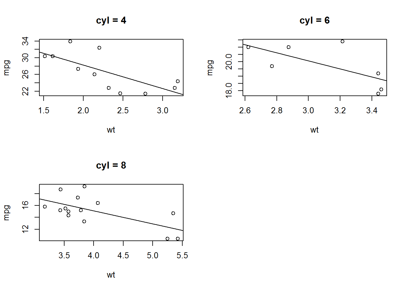
4. 帮助函数
帮助函数都是一些函数运算符,输入函数,包装为另一个函数。
4.1 splat()
将一个需要多个参数的函数转变为需要一个列表作为单一参数的函数。这在计算数据框时很有用,列名自动匹配函数中的参数名。
hp_per_cyl <- function(hp, cyl, ...) hp/cyl
splat(hp_per_cyl)(mtcars[1,])
## [1] 18.33333splat(hp_per_cyl)(mtcars)## [1] 18.33333 18.33333 23.25000 18.33333 21.87500 17.50000 30.62500
## [8] 15.50000 23.75000 20.50000 20.50000 22.50000 22.50000 22.50000
## [15] 25.62500 26.87500 28.75000 16.50000 13.00000 16.25000 24.25000
## [22] 18.75000 18.75000 30.62500 21.87500 16.50000 22.75000 28.25000
## [29] 33.00000 29.16667 41.87500 27.25000dlply(mtcars,.(round(wt)),function(df) hp_per_cyl(df$hp, df$cyl))## $`2`
## [1] 23.25 16.50 13.00 16.25 24.25 16.50 22.75 28.25
##
## $`3`
## [1] 18.33333 18.33333 18.33333 21.87500 17.50000 15.50000 23.75000
## [8] 20.50000 20.50000 18.75000 33.00000 29.16667 27.25000
##
## $`4`
## [1] 30.625 22.500 22.500 22.500 18.750 30.625 21.875 41.875
##
## $`5`
## [1] 25.625 26.875 28.750
##
## attr(,"split_type")
## [1] "data.frame"
## attr(,"split_labels")
## round(wt)
## 1 2
## 2 3
## 3 4
## 4 5dlply(mtcars,.(round(wt)),splat(hp_per_cyl))## $`2`
## [1] 23.25 16.50 13.00 16.25 24.25 16.50 22.75 28.25
##
## $`3`
## [1] 18.33333 18.33333 18.33333 21.87500 17.50000 15.50000 23.75000
## [8] 20.50000 20.50000 18.75000 33.00000 29.16667 27.25000
##
## $`4`
## [1] 30.625 22.500 22.500 22.500 18.750 30.625 21.875 41.875
##
## $`5`
## [1] 25.625 26.875 28.750
##
## attr(,"split_type")
## [1] "data.frame"
## attr(,"split_labels")
## round(wt)
## 1 2
## 2 3
## 3 4
## 4 54.2 each()
each接收并运算多个函数
ddply(mtcars,"cyl",summarise,MM=each(min,max)(mpg))## cyl MM
## 1 4 21.4
## 2 4 33.9
## 3 6 17.8
## 4 6 21.4
## 5 8 10.4
## 6 8 19.2ddply(mtcars,"cyl",summarise,M1=min(mpg),M2=max(mpg))## cyl M1 M2
## 1 4 21.4 33.9
## 2 6 17.8 21.4
## 3 8 10.4 19.24.3 colwise()
将一个用在vector上的函数转变为按列应用在数据框上的,有参数.if = is.factor或if = is.numeric。
mtcars1 <- mtcars
mtcars1$cyl <- factor(mtcars$cyl)
mtcars1$vs <- factor(mtcars$vs)
mtcars1$am <- factor(mtcars$am)
mtcars1$gear <- factor(mtcars$gear)
mtcars1$carb <- factor(mtcars$carb)numcolwise(mean)(mtcars1)## mpg disp hp drat wt qsec
## 1 20.09062 230.7219 146.6875 3.596563 3.21725 17.84875colwise(pryr::compose(length,unique))(mtcars[sapply(mtcars1, is.factor)])## cyl vs am gear carb
## 1 3 2 2 3 64.4 failwith()
将一个函数抛出错误变为返回某值
failwith(NA,function(x,y) x+y,quiet = T)("1","2")## [1] NA4.5 as.data.frame.function()
将一个函数返回值强制转变为DataFrame型
4.6 summarize()
- transform函数返回变更一列或添加新列的原始数据;
- summarise函数返回一个新的数据框,包含更改或新列;
ddply(mtcars[1:3],"cyl",transform, A = mpg+1) %>% nrow()## [1] 32ddply(mtcars[1:3],"cyl",summarise, A = mean(mpg))## cyl A
## 1 4 26.66364
## 2 6 19.74286
## 3 8 15.100004.7 .progress参数
- “none”不显示进度
- “text”显示文本进度
5. 策略
通用流程:
- 抽取数据子集以方便解决问题;
- 手动解决子问题,并检验计算结果;
- 写一个能解决该子问题的函数;
- 在原始数据上使用plyr函数,来应用在每一部分;
5.1 案例一:棒球
dim(baseball)## [1] 21699 22names(baseball)## [1] "id" "year" "stint" "team" "lg" "g" "ab" "r"
## [9] "h" "X2b" "X3b" "hr" "rbi" "sb" "cs" "bb"
## [17] "so" "ibb" "hbp" "sh" "sf" "gidp"取四列
baseballs <- baseball[,c("id","year","rbi","ab")]取某个运动员的数据子集
baberuth <- subset(baseballs, id == "ruthba01")计算此运动员的从职业生涯开始到那场比赛的年数
baberuth <- transform(baberuth, cyear = year - min(year) + 1)那么对于所有运动员,可以这么算
baseball <- ddply(baseballs, "id", transform, cyear = year - min(year) + 1)
names(baseball)
## [1] "id" "year" "rbi" "ab" "cyear"对于每一个投手,计算rbi/ab随cyear变化的规律
plot(baberuth$cyear,baberuth$rbi/baberuth$ab,type = "l")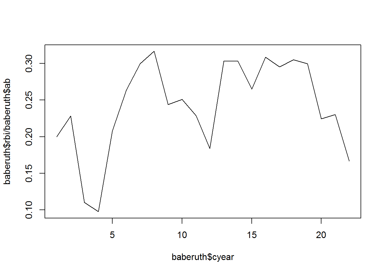
baseball <- subset(baseball, ab >= 25)
xlim <- range(baseball$cyear, na.rm=T)
ylim <- range(baseball$rbi/baseball$ab,na.rm=T)
plotpattern <- function(df){
  qplot(cyear,rbi/ab,data=df,geom="line",
        xlim=xlim,ylim=ylim)
}
pdf("paths.pdf",width = 8,height = 4)
#d_ply(baseball,.(reorder(id, rbi/ab)),failwith(NA,plotpattern),.print=T,.progress = "text")
dev.off()
## png
## 2图中似乎看不出什么规律
所以考虑用线性回归拟合模型
model <- function(df){
  lm(rbi / ab ~ cyear,data=df)
}model(baberuth)##
## Call:
## lm(formula = rbi/ab ~ cyear, data = df)
##
## Coefficients:
## (Intercept) cyear
## 0.203200 0.003413summary(model(baberuth))$r.squared## [1] 0.1240673拟合所有的运动员,得到1152个模型
bmodels <- dlply(baseball,"id",model)
length(bmodels)
## [1] 1152提取参数和R方项
rsq <- function(x) summary(x)$r.squared
bcoefs <- ldply(bmodels,function(x) c(coef(x),rsquare=rsq(x)))
names(bcoefs)[2:3] <- c("intercept","slope")
head(bcoefs)
## id intercept slope rsquare
## 1 aaronha01 0.18329371 0.0001478121 0.000862425
## 2 abernte02 0.00000000 NA 0.000000000
## 3 adairje01 0.08670449 -0.0007118756 0.010230121
## 4 adamsba01 0.05905337 0.0012002168 0.030184694
## 5 adamsbo03 0.08867684 -0.0019238835 0.108372596
## 6 adcocjo01 0.14564821 0.0027382939 0.229040266qplot(rsquare,data=bcoefs,geom="histogram")## `stat_bin()` using `bins = 30`. Pick better value with `binwidth`.## Warning: Removed 1 rows containing non-finite values (stat_bin).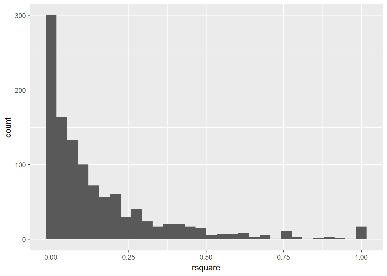
大多数R方都不理想,有少部分接近于1,提取那部分
baseballcoef <- merge(baseball,bcoefs,by="id")
subset(baseballcoef,rsquare > 0.999)$id %>% table()
## .
## bannifl01 bedrost01 burbada01 carrocl02 cookde01 davisma01 jacksgr01
## 2 2 2 2 2 2 2
## lindbpa01 oliveda02 penaal01 powerte01 splitpa01 violafr01 wakefti01
## 2 2 2 2 2 2 2
## weathda01 woodwi01
## 2 2所有拟合地好的模型都只有两个点
g <- ggplot(bcoefs,aes(slope,intercept))+
  geom_point(aes(size=rsquare),colour="steelblue",alpha=0.5)+
  geom_hline(yintercept = 0)+geom_vline(xintercept = 0)
g
## Warning: Removed 25 rows containing missing values (geom_point).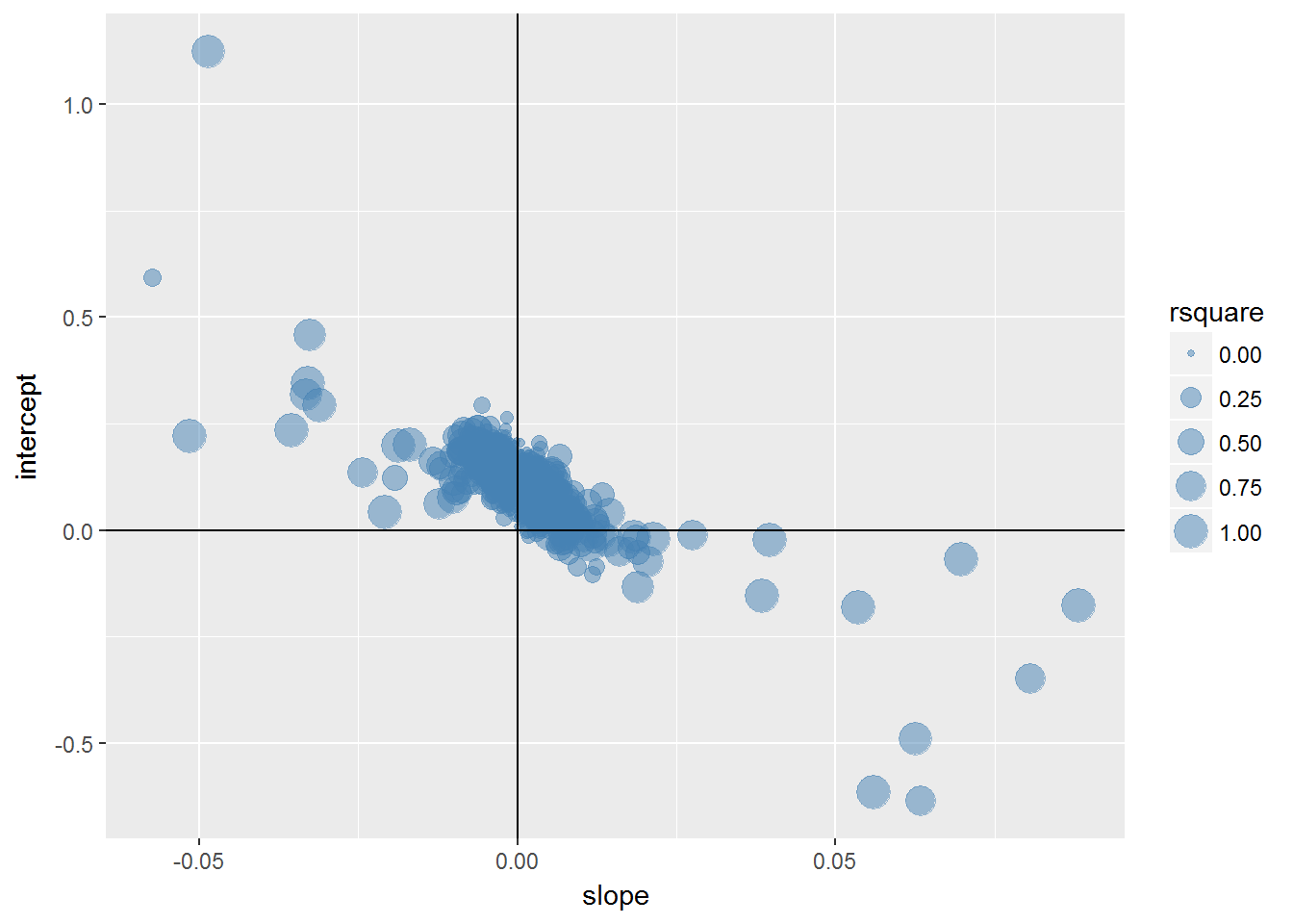
g+xlim(c(-0.01,0.01))+ylim(c(-0.1,0.25))## Warning: Removed 82 rows containing missing values (geom_point).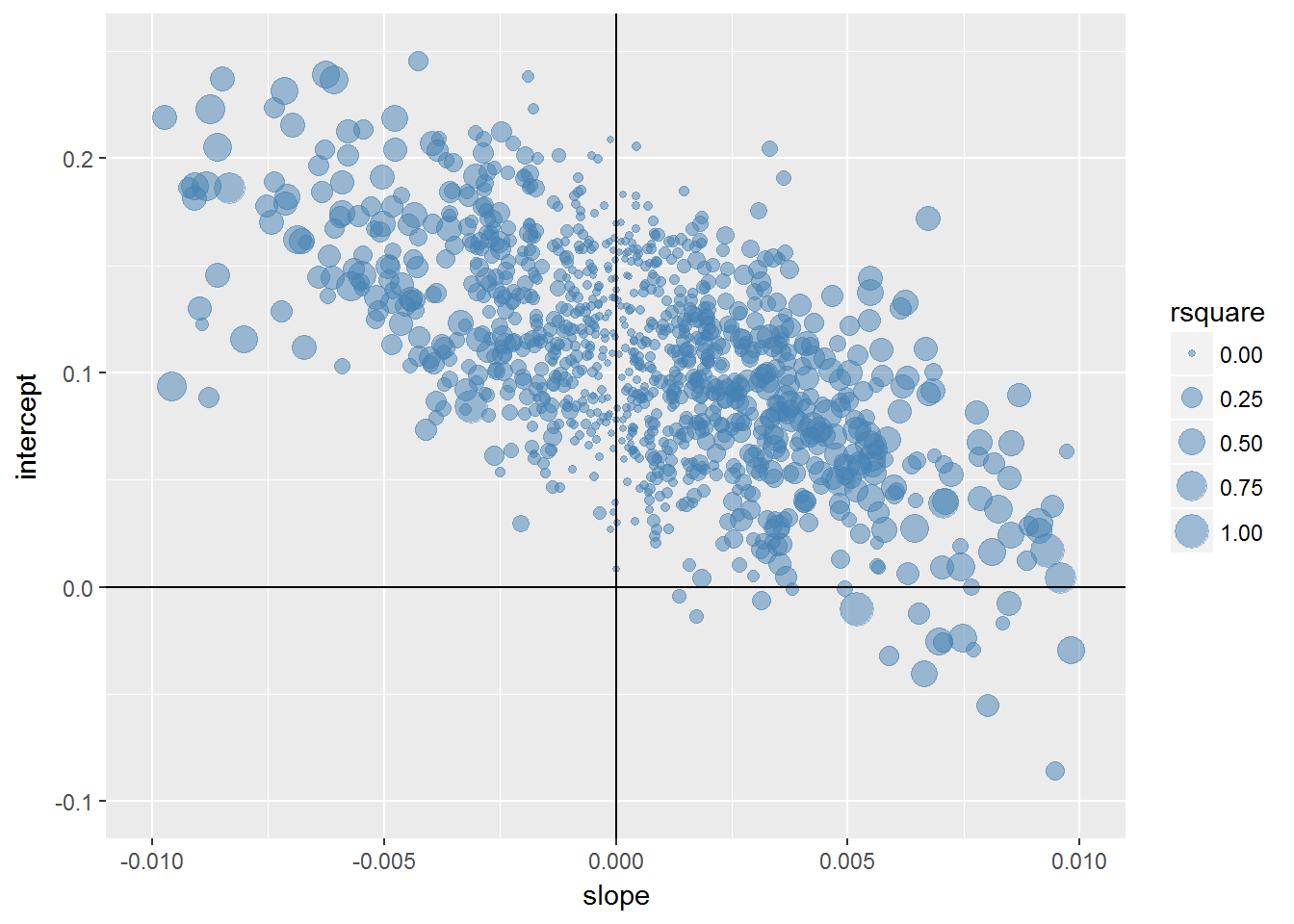
R方小的模型,斜率靠近0。
5.2 案例二:臭氧层
待补充…
7. 总结
plyr包是非常精心设计的,速度非常快,内存使用尽可能最小了。未来还将加入foreach包,来实现多核和多机器计算。
怎样识别其他的通用计算模式?能后退一步来识别这些模式非常难,因为我们很容易被计算的细节所迷惑,而通用的理念变得模糊了。认识到“分而治之”的策略花了Wickham四年的时间,但他认为这个工作很有必要,因为让数据分析变简单了。